Building a Model
|
Topics: |
In this section, we will review the different model types that are available in RStat and build a Decision Tree model. For more information, see Building the Decision Tree Model.
Model Tab Options
|
Topics: |
|
How to: |
Using RStat, you can define and execute various models against a selected database.
Note:
- Depending on your data, certain model types may be disabled.
- The Ada Boost option is selected by default.
- You can click Select All to select all relevant models, or select one or multiple models to perform a simultaneous analysis. To view the output of other models that were selected for simultaneous execution, click the model type within the Model Type table.
The supported model types and their exportability are listed in the following table.
|
Model Type |
Exportability |
|---|---|
|
Ada Boost |
C Exportable(.c);PMML Exportable(.xml) |
|
ARIMA |
None |
|
Bayesian Network |
None |
|
Binomial Regression |
C Exportable(.c);PMML Exportable(.xml) |
|
Decision Tree |
C Exportable(.c);PMML Exportable(.xml) |
|
Gamma Regression |
C Exportable(.c);PMML Exportable(.xml) |
|
Gaussian Regression |
C Exportable(.c);PMML Exportable(.xml) |
|
Inverse Gaussian Regression |
C Exportable(.c);PMML Exportable(.xml) |
|
Linear Regression |
C Exportable(.c);PMML Exportable(.xml) |
|
Logistic Regression |
C Exportable(.c);PMML Exportable(.xml) |
|
Multinomial Regression |
C Exportable(.c);PMML Exportable(.xml) |
|
Negative Binomial |
C Exportable(.c);PMML Exportable(.xml) |
|
Neural Net |
C Exportable(.c);PMML Exportable(.xml) |
|
Poisson Regression |
C Exportable(.c);PMML Exportable(.xml) |
|
Random Forest |
C Exportable(.c);PMML Exportable(.xml) |
|
Survival |
C Exportable(.c);PMML Exportable(.xml) |
|
SVM |
PMML Exportable(.xml) |
The following procedure provides basic guidance for executing a model type option.
Procedure: How to Execute a Model Type Option
- Open RStat.
- Click the folder adjacent to the Filename field and select a data set.
- Click Execute to load the data.
- Click the Model tab.
- Select a model type.
- Select or populate fields based on the model type that you select. For more information, refer to each of the model options discussed in this section.
- Click Execute to
view the model based on your selections.
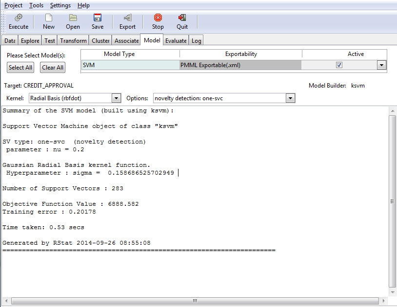
For example, the following image illustrates the results of modeling using SVM with the default Kernel value selected (Radial Basis (rbfdot)). The novelty detection: one-svc option was selected.
The following sections present key functionality for each of the different model types.
Ada Boost Model
The Ada Boost model uses the ada, which is the underlying algorithm (model builder). Boosting builds multiple, but generally simple, models. The models might be decision trees that have just one split. These are commonly referred to as decision stumps.
Note:
- The Ada Boost model returns class and probability.
- Ada Boost is for non-regression binary trees.
The Boost model allows you to specify the number of trees, in addition to other criteria, as shown in the following image.
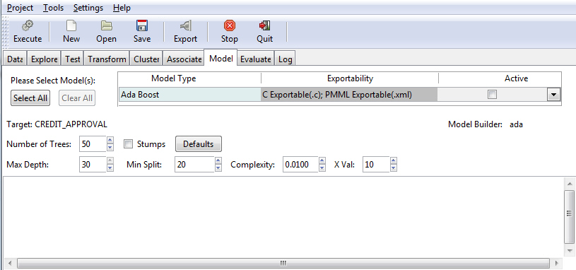
The following table lists and describes the fields that are used to adjust the Boost model.
|
Field Name |
Description |
|---|---|
|
Number of Trees |
The number of trees to build. Note: In order to ensure that every input row is predicted at least a few times, this value should not be set to a number that is too low. The default value is 50. |
|
Max Depth |
Allows you to set the maximum depth of any node of the final tree. The root node is counted as depth 0. The default value is 30. Note: Values greater than 30 will generate invalid results on 32-bit machines. |
|
Stumps |
If the Stumps check box is selected, you can build stumps using the Boost model. If the Stumps check box is not selected, the results in the default values are deactivated. |
|
Min Split |
The minimum number of entities that must exist in a data set at any node for a split of that node to be attempted. The default value is 20. |
|
Complexity |
Also known as the complexity parameter (cp), this value allows you to control the size of the decision tree and select the optimal size tree. If the cost of adding another variable to the decision tree from the current node is above the value of the cp, then tree building does not continue. The default value is 0.0100. Note: The main role of this parameter is to save computing time by pruning unnecessary splits. |
|
X Val |
Refers to the number of cross-validation errors allowed. The default value is 10. |
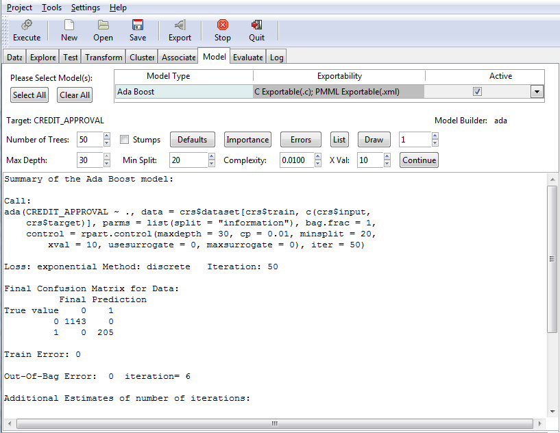
Once you have defined your model criteria, you must click the Execute button to review the results, as shown in the following image.
ARIMA Model
The Autoregressive Integrated Moving Average (ARIMA) model is used for short term forecasting. Also known as Box-Jenkins, ARIMA is used with data sets that show a stable, consistent pattern over time. The general idea of the model is to be able to forecast future values based on the patterns of the data points used in the current data set.
ARIMA requires at least 40 historical data points to forecast the future values in a series. The model works best when your data reveals a consistent pattern with few outliers.
Once you select ARIMA as the model, you must click Execute to load the ARIMA Forecasting GUI, as shown in the following image.
The following table lists and describes the fields that are used when working with an ARIMA model.
|
Field Name |
Description |
|---|---|
|
DATA |
|
|
Check Data: |
Summary and Plot. Provides a summary of the data that has been loaded. It displays the first few records of the data set, along with a summary of the variable to be forecasted: minimum, first quartile, median, mean, third quartile, and maximum. The plot is a time series. |
|
TRANSFORMATION |
|
|
Trans. Method |
Select the transformation method used when you click the Transformation button. You can select from the following options:
|
|
Check Trans. |
Creates a new vector or data column using the selected transformation on the historical data. |
|
BUILD ARIMA |
|
|
Auto Arima: |
Runs the Auto ARIMA function and returns the best ARIMA model according to either AIC, AICc, or BIC. |
|
Check ACF, PACF |
ACF and PACF compute and plot the autocorrelation and partial autocorrelation functions, respectively. You can select from the following options:
|
|
Construct Arima: |
Allows you to enter user-defined values for the arguments p, d, and q. When you execute the model the first time, it is saved in memory as ARIMA_1. All consecutive executions are named ARIMA_n, where n is the next consecutive number assigned. You can populate values for the following fields:
|
|
MODEL DIAGNOSE |
|
|
Select Model |
Lists the models that you have generated while using the Construct Arima section. Click Show Summary to display the ARIMA model summary. |
|
Check Residuals |
Produces a time plot of the residuals, the corresponding ACF, and a histogram. You can select from the following options:
|
|
Box. Test |
Compute the Box-Pierce or Ljung-Box test for examining the null hypothesis of independence in a given time series. Options include:
|
|
EXPORT |
|
|
What to Export: |
Provides options for exporting modeling information. Options include:
|
Bayesian Network Model
|
Topics: |
Bayesian networks, also known as belief networks (or Bayes nets), are a type of probabilistic graphical model. They can be used to make predictions and automated insights, and perform diagnostics. It represents a set of random variables and their conditional dependencies, thus it allows you to represent and reason about uncertainties.
Bayesian networks are directed acyclic graphs (DAGs), which use random variables to represent observable quantities or hypotheses. Each graph has nodes, which represent these random variables, one node per variable. The edges between the nodes represent conditional dependencies amongst the variables.
Note: When working with the Bayesian model and the data is loaded, no variable should be selected as target; all variables should be selected as input.
The Bayesian network model is effective in illustrating probability through the use of graphs and the variables that comprise them. The Bayesian Network options are shown in the following image.
The following table lists and describes the tabs and fields that are used when working with the Bayesian model.
|
Tab Name |
Field Name |
Description |
|---|---|---|
|
Preparing Data |
The following fields display:
|
When loading variables with a Categoric data type, the Preparing Data tab will be disabled. When loading variables with a Numeric data type, the Preparing Data tab will be enabled and the Discretize Data button will be available. When you click this button, the selected variables are divided into intervals, converting continuous data into discrete data. The Preparing Data tab will initially display a summary of the loaded variables. This summary assists in the setting of intervals for discretizing the data. On this tab:
If Set Labels is left blank, then the actual interval will be displayed. For example, (70,90]. If you want to use labels, use the R syntax. For example, c(1,2,3) or c("A","B","C"). The number of labels must be one less than the number of values used when setting the intervals. For example, in the intervals c(30,50,70,90) are four values. Exactly three labels must be entered. |
|
Structure Learning |
The following field displays:
|
In simple cases, an expert can specify a Bayesian network used to perform inference. In more complex cases, the network structure and the parameters of the local distributions must be learned from the data. You can use the following steps to specify a learning algorithm:
The learning is displayed in the text view and the network is displayed in a separate R graphics window. Note: A new R graphics window is opened every time you click Execute. |
|
Parameter Estimation |
The following fields display:
|
In a distribution model, the set of parameters needs to be estimated. These parameters specify any constants in the model, enabling efficient and accurate use of the data. For the parameter estimation to work correctly, the network must be a directed acyclic graph (DAG), as plotted on the Structure Learning tab. If the graph is not a DAG, then the following error message will display: the graph is only partially directed. |
|
Inference |
The following fields display:
|
The Inference tab is used to perform conditional probability queries (CPQs). If the query type is Probability, then enter the event of interest as fieldname=="factor level". Evidence is enter as fieldname=="factor level". If the query type is Observations, then enter the event of interest as "fieldname". Evidence is entered fieldname=="factor level'. |
Plotting Conditional Probability
- Click the Structure Learning tab and select and execute a learning algorithm, for example Hill-Climbing.
- Click the Parameter Estimation tab and select and execute a Method. For example, Maximum Likelihood parameter estimation (mle).
- Then, on the Inference tab, click the Observations radio button. For Event, enter any one of the variable names in quotes. For example, "STAT". For Evidence, enter a logical statement, for example, VECT >= 50. To run an unconditional probability distribution, set either event or evidence to TRUE.
- Click Plot.
- A histogram displays, showing the frequency distribution.
Note: Before the plot is generated, the parameters of the Bayesian network are fitted conditional on its structure and random observations conditional on the evidence using the logic sampling method are generated.
A sample plot is shown in the following image.
Bayes Factor Analysis
After loading the data and selecting a target, you can perform a Bayes factor analysis. From the Model tab, select Linear Regression and click Execute. Click Bayesian Linear Analysis, which displays the Bayes Factor Analysis of Regression user interface and simultaneously computes Bayes factors for groups in regression designs, as shown in the following image.
Note: There are three icons that consistently display when using the Bayes Factor Analysis GUI: the brush, which will clear the output areas Textview and Comparison Plot, the disc icon, which will save the current plot in the following formats: .pdf, .png, .jpg, and .wmf, and the pipe connector icon, which exports the content of the Textview pane.
|
Tab Name |
Field Description |
|---|---|
|
General Linear Regression |
Specified Model. The specified model contains the formula for computing Bayes factors for a linear regression model. Show Selected Model. Enter the formula into the Edit text box and then click Specified Model. This adds the model to the Show Selected Model drop-down list box, making it available for selection. Select a model from the drop-down list and click Show Selected Model, which will display the Bayes factor analysis for the selected model in the Textview pane. Example formulas include: len~supp and len~dose+supp. |
|
Regression(Numeric) |
The following buttons display in the Bayes Factor Analysis GUI: Best Models. Click this button to show the best six models in the Textview pane. This also shows the Bayes Factor Analysis along with the name of the model. Worst Models. Click this button to show the worst six models in the Textview pane. This also shows the Bayes Factor Analysis along with the name of the model. All Models. Click this button to show all models without the Bayes factor analysis. Specified Model. Retype or copy and paste any one of the model names from the All Models in Textview. Ensure that when you enter this into the text box, the model name is enclosed in quotes. For example, "complaints + privileges", and then click the Specified Model button to display the Bayes Factor Analysis. Comparison Plot. There are three types of comparison plots: Best Model (all), Most Complex Model (top), and Intercept Only (bottom). Clicking this will update both the Textview pane and the Comparison Plot pane. |
Decision Tree Model
The Decision Tree option is used to generate a decision tree, which is the prototypical data mining technique. It is widely used because of its ease of interpretation. The Decision Tree model uses an underlying algorithm (model builder) of rpart, as shown in the following image.
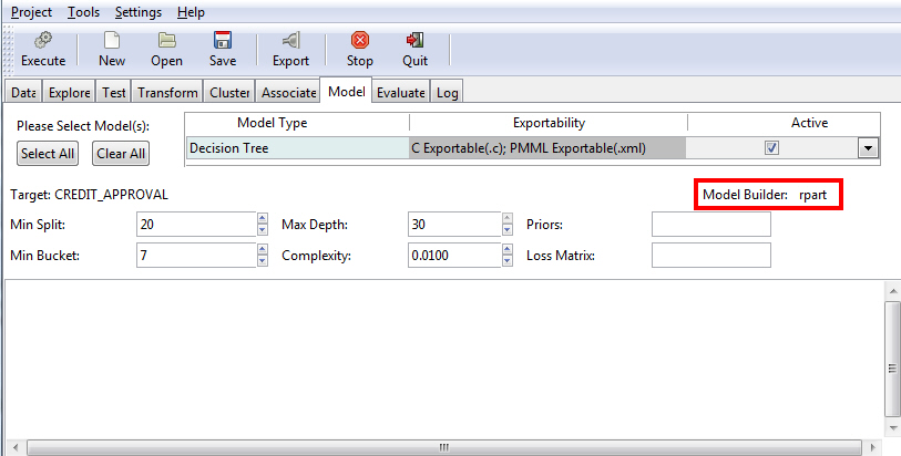
The following table lists and describes the fields that are used to adjust a Decision Tree model.
|
Field Name |
Description |
|---|---|
|
Min Split |
The minimum number of entities that must exist in a data set at any node for a split of that node to be attempted. The default value is 20. |
|
Min Bucket |
The minimum number of entities allowed in any leaf node of the decision tree. The default value is one third of the min split. |
|
Max Depth |
Allows you to set the maximum depth of any node of the final tree. The root node is counted as depth 0. The default value is 30. Note: Values greater than 30 will generate invalid results on 32-bit machines. |
|
Complexity |
Also known as the complexity parameter (cp), this value allows you to control the size of the decision tree and select the optimal size tree. If the cost of adding another variable to the decision tree from the current node is above the value of the cp, then tree building does not continue. The default value is 0.0100. Note: The main role of this parameter is to save computing time by pruning unnecessary splits. |
|
Priors |
Allows you to set the prior probabilities for each class. |
|
Loss Matrix |
Allows you to weight the outcome classes differently. |
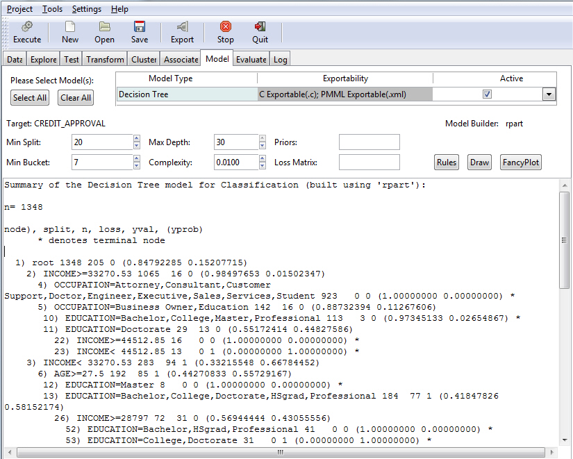
Once you have specified your model criteria, you must click the Execute button to view the result. Since Tree was selected, the Summary of the Decision Tree model displays, as shown in the following image.
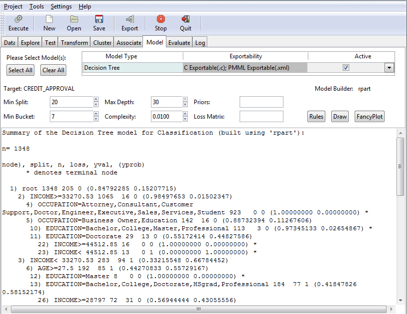
Note: The default values for all fields were used to create this example.
You can view the summary or access other features of the application, including Rules, Draw, and FancyPlots. For more information, see:
Regression Model
Regression is a traditional approach to modeling. The model builder glm (logit) is used by the Regression model. Logistic regression (using the binomial family) is used to model binary outcomes. Linear regression is used to model a linear numeric outcome. For predicting where the outcome is a count, the Poisson family is used. Generalized Regression is generalization of standard linear regression, allowing for response variables that fall outside of a normal distribution. Multinomial regression generalizes logistic regression, in that it allows more than two discrete outcomes. For more information, see Building a Logistic Model and Building a Linear Regression Model.
RStat supports regression and advanced regression, as shown in the following image.
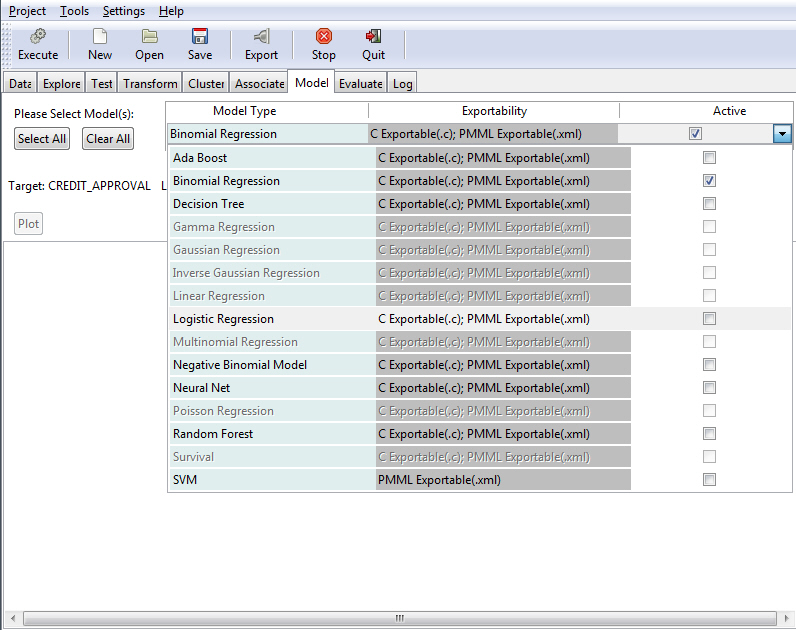
The following techniques related to regression can be performed:
- Binomial. Distribution is binomial distribution, which is a discrete probability distribution of the number of successes in a sequence of a variable number (n) of dependent Yes or No experiments. The LinkFunction could be either logit, probit, or cauchit.
- Gamma. The error distribution is Gamma distribution. The LinkFunction could be inverse, identity, or log.
- Gaussian. The error distribution is normally distributed. The response method is dependent on the LinkFunction. The LinkFunction can be identity, log, or inverse.
- Inverse Gaussian. The error distribution is Gamma distribution. The LinkFunction could be inverse, identity, log, or 1/mu^2.
- Linear. The error distribution is normally distributed. The response variable is linear in relation to the predictive model.
- Logistic. Usually referred to as binomial or binary logistic regression, this is used to predict two possible types of outcome (YES or NO).
- Multinomial. Referred as multinomial logistic regression, this is used to predict three or more possible types of outcome.
- Negative Binomial. The error distribution is negative binomial distribution, which is a discrete distribution of the number of successes in a sequence of Bernoulli trials before a specified number of failures occur.
- Poisson. The error distribution or response variable distribution is Poisson distribution. Poisson regression is used to model and predict in cases where count data and contingency tables are used.
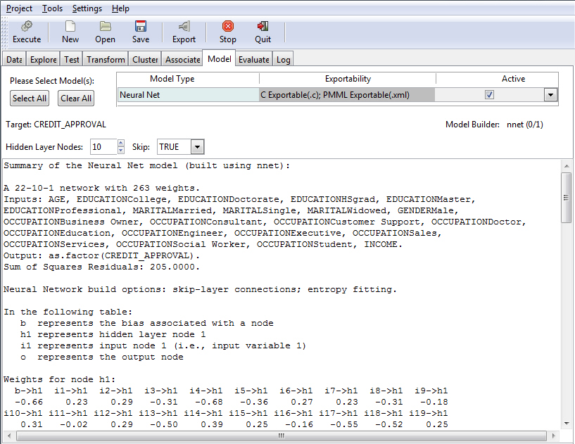
Neural Net Model
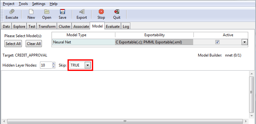
Neural Network (Neural Net) is an older approach to modeling. The Neural Net model uses a structure that resembles the neural network of a human being. When applied to modeling, the concept is to build a network of neurons that are connected by synapses. Rather than generate electrical signals, however, the network propagates numbers.
When using the Neural Net model, you can include or exclude the interval of networks from your model. The interval of networks is used to define and describe the relationships within your model. Display of these intervals is accomplished using the Skip field. When set to True (default), the interval of networks displays. If the Skip field is set to False, the interval of networks does not display.
The default value of True is shown in the following image.
The following table lists the options that are available on the Neural Net model screen.
|
Field Name |
Description |
|---|---|
|
Hidden Layer Nodes |
The number of hidden layer nodes to display. The default is 10. |
|
Skip |
Set to a value of TRUE by default, this field switches between the input and output of skip-layer connections, depending on your selection. |
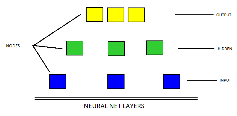
In the following diagram, the relationships between the different layers of a neural record are illustrated. The bottom portion represents the input layer, the middle nodes form the hidden layer, and the top components constitute the output layer.
Note: The number of nodes varies in different applications. In addition, you must have a data set selected and loaded in order to use this functionality.
The following example shows the results of a Neural Net model with the Skip field set to True. Accordingly, RStat displays the interval of networks.
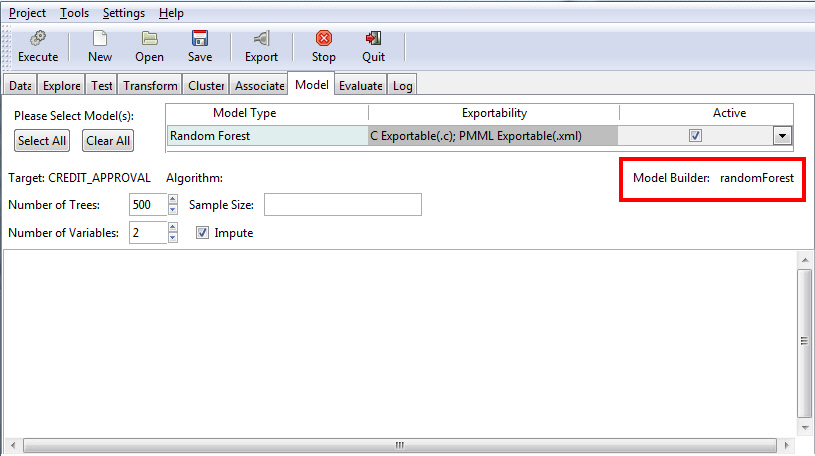
Random Forest Model
The Random Forest uses an underlying algorithm (randomForest), which builds multiple decision trees from different samples of the data set. While building each tree, random subsets of the available variables are considered for splitting the data at each node of the tree.
Note:
- When using the C export with the Random Forest model, class and regression(numeric values) are returned.
- Random Forest trees can be binary and k-ary(k>2).
You can specify a number of trees (the default is 500) and a number of variables (the default is 4), as shown in the following image.
The following table lists and describes the fields that are used to adjust the Random Forest model.
|
Field Name |
Description |
|---|---|
|
Number of Trees |
The number of trees to build. Note: In order to ensure that every input row gets predicted at least a few times, this value should not be set to a number that is too low. The default value is 500. |
|
Number of Variables |
This is the number of variables to be considered at any time in deciding how to partition the data set. Each split produces a number of variables which are randomly sampled as candidates. |
|
Sample Size |
Size(s) of a sample to draw. |
|
Impute |
This applies to missing variables. If this check box is selected, the variables are transferred by replacing any NA values with one of the following (depending on the current selection):
|
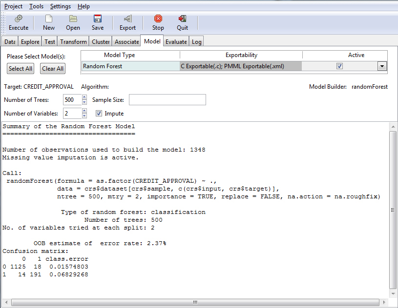
Once you have indicated your criteria, you must click the Execute button to see the results, as shown in the following image.
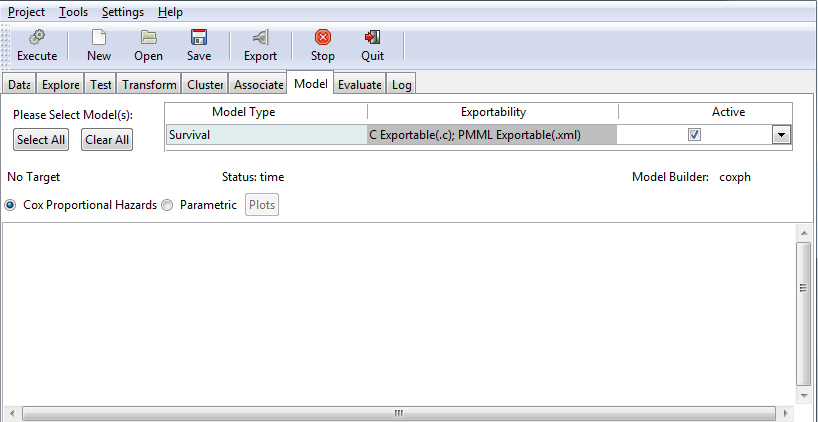
Survival Model
The Survival Model is used to model time-to-event data. When using this option, you can select Cox Proportional Hazards (coxph) or Parametric (survreg) to perform your Survival Analysis, as shown in the following image. For more information on the Survival model, see Building a Survival Model.
The following table lists and describes the fields that are used to adjust a Survival model.
|
Field Name |
Description |
|---|---|
|
Time |
The variable that you selected (time) on the Data tab. |
|
Status |
The variable that you selected (status) on the Data tab. |
|
Model Builder |
The name of the model builder (coxph or survreg) related to the selection you made: Cox Proportional Hazards or Parametric. |
|
Cox Proportional Hazards |
A general regression model that predicts individual risk relative to the population. |
|
Parametric |
Also known as the accelerated failure time model, this regression model predicts the expected time to the event of interest. |
|
Survival |
This option enables you to view the results of the Cox Proportional Hazards model. For more information, see Building a Survival Model. |
|
Residuals |
This button enables the testing of the assumption of proportional hazards. |
SVM Model
The Support Vector Model (SVM) is a modern approach to modeling where the data is mapped to a higher dimensional space. This increases the possibility that vectors separating the classes will be found.
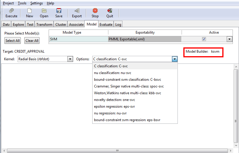
You can select the SVM option to specify a kernel and related options in support of the model.
Note:
- The kernel functions are from the SVM defines. Type ksvm can be used for classification, regression, or novelty detection.
- The list of options is the same for all kernels.
The Options drop-down list defaults to C classification: C-svc, as shown in the following image. If you do not make a selection from the Options drop-down list, the default value is used.
The following table lists the options that are available on the SVM model screen.
|
Field Name |
Description |
|---|---|
|
Kernel |
The kernel function is used in training and predicting. You can select one of the following kernels:
|
|
Options |
The ksvm model builder can be used for classification, regression, or novelty detection. When using the ksvm model builder, you can select one of the following options from the drop-down list:
|
Building the Decision Tree Model
This section reviews the basic procedure for building a Decision Tree model.
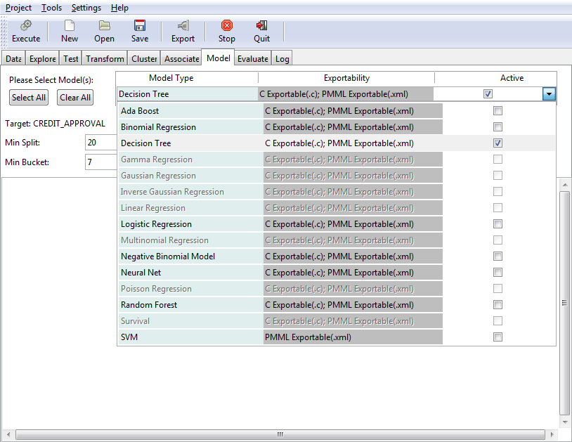
- Select the Model tab.
- From the Model Type
drop-down list box, select Decision Tree,
as shown in the following image.
- Click Execute to
create the model.
The model metadata or output appears in the model textview area, as shown in the following image.
Visualizing the Decision Tree Model
|
Topics: |
|
How to: |
The Decision Tree generates rules that predict the score and divides the sample data into multiple segments (branches). Each branch terminates in a node that associates a subset of the customers with a predicted score. The rules describe the criteria that qualify for each node. The predicted score is a probability value between 0 and 1. Those with a probability of .5 or greater are predicted as a good risk, and those with less than .5 are predicted as a bad risk.
You can display the rules or diagram the nodes.
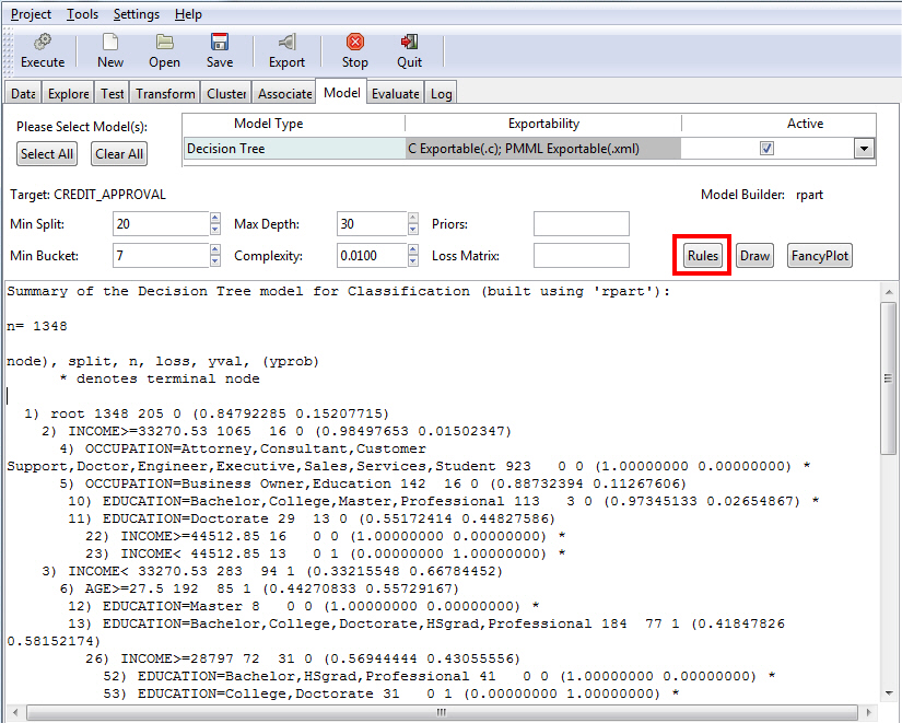
Procedure: How to Display the Decision Tree Model Rules
- On the Model
tab, click Rules to display the rules associated
with the selected database, as shown in the following image.
The Rpart Rules GUI displays, as shown in the following image.
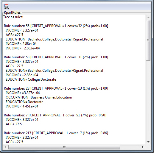
- Scroll down to review the rules.
- Optionally,
click Save current output to file to save
the rules information as a .txt or .xml file.
The Export Rpart Rules dialog displays, as shown in the following image. This enables you to specify a file name and a folder location.
Note: You can save the file in the current (default) folder or specify a new folder in which to place the file by clicking Browse for other folders.
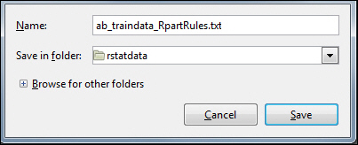
- Click Save to save the file.
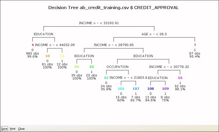
Procedure: How to Diagram the Decision Tree Model Rules
- On the Model
tab, click the Draw button, as shown in the following image.
The diagram displays in the RGui.
The colored numbers at the end of each node correspond to the rules, as shown in the following image.
Using FancyPlots
|
Topics: |
|
How to: |
Accessed from the Model tab in the RStat application, the FancyPlot functionality enables you to plot data from the database with which you are working. You can also split the plot or collapse nodes in the tree. FancyPlots provide unique charting options that can be customized for each data set.
Procedure: How to Access FancyPlots
- Launch RStat.
- On the Data tab, select a file name to load and then click Execute.
- On the Model tab, from the Model Type list, click Decision Tree and then click Execute.
- Click FancyPlot,
as shown in the following image.
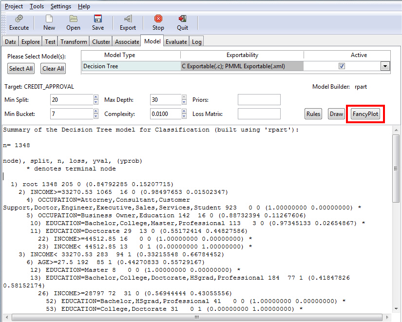
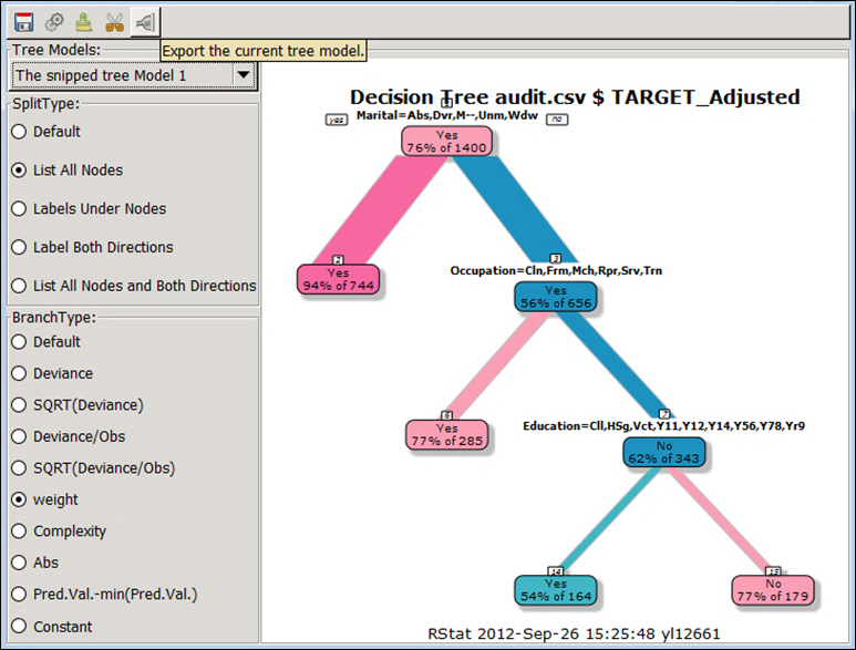
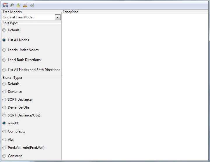
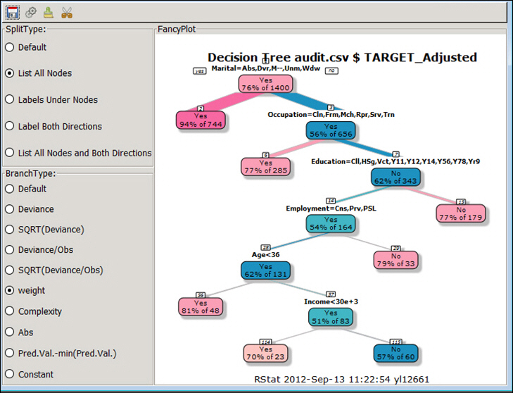
The FancyPlot functionality displays, as shown in the following image.
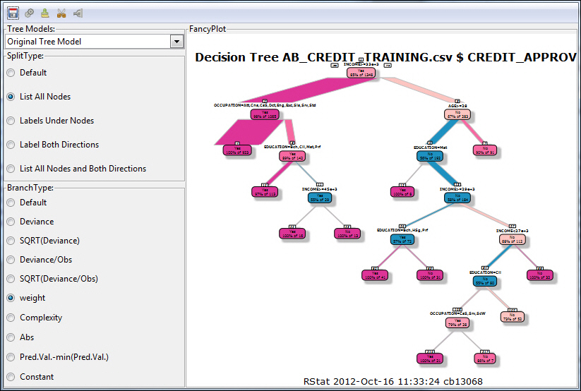
You can use varying combinations in the primary sections: SplitType and BranchType. Upon selecting different combinations of type and branch, click Execute in the toolbar to update the tree image in the drawing area.
The following table defines these options.
Group
Field
Description
SplitType
Default
The default. Draw a split label at each split and a node label at each leaf.
List All Nodes
Label all nodes, not just the leaves. Similar to text.rpart all=TRUE.
Labels Under Nodes
Similar to List All Nodes, but draws the split labels below the node labels. Similar to the plots in the CART book.
Label Both Directions
Draw separate split labels for the left and right directions.
List All Nodes and Both Directions
Similar to Label Both Directions, but labels all nodes, not just leaves.
BranchType
Default
The default. The branch lines are drawn conventionally.
Deviance
Deviance
SQRT(Deviance)
Square-root (deviance)
Deviance/Obs
Deviance / nobs
SQRT(Deviance/Obs)
The standard deviation when method=anova
weight
Also known as frame$wt, this is the number of observations at the node, unless rpart weight argument was used.
Complexity
Abs
This is the predicted value.
Pred.Val.-min(Pred.Val.)
Constant
For checking visual perception of the relative width of branches.
The GUI also has a toolbar with options that enable some of the basic functionality of charting. From left to right, these options are: Save current output to file, Execute current selections, Clear output area, Collapse nodes and re-plot model, and Export the current tree model.
Charting With FancyPlots
You can use any combination of Split Type and Branch Type to build your chart. You can clear the output area before creating a new chart or work with the initial chart that displays by default. You can perform the following tasks when charting with FancyPlots:
- Click Save current output to file to save the current image.
- Click Execute current selections to update the image with the current setting or show the selected snipped model.
- Click Collapse nodes and re-plot mode to enable the Snipping function.
- Click Clear output area to clear the drawing area.
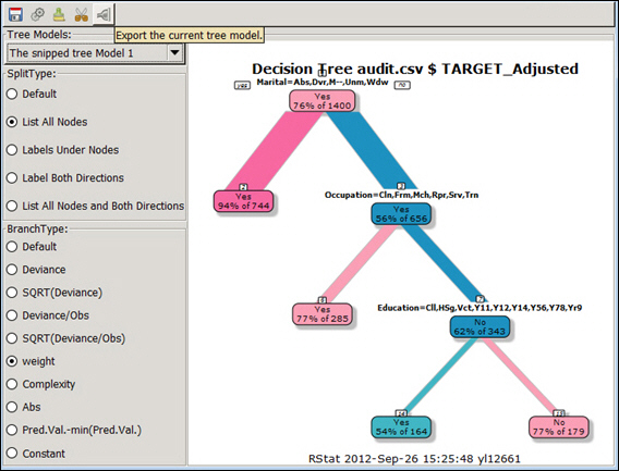
- Click Export the current tree model to export the selected (current) tree model as a scoring routine.
Some additional concepts for charting with FancyPlots include:
- You can collapse nodes in the tree using the scissors icon, which is available in the toolbar.
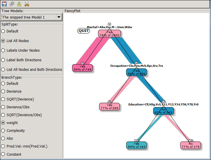
- When the plot is active, you will see a Quit option in the upper-left corner of the chart and all nodes will be connected with black lines.
- When you click on a node, the subtree will be colored.
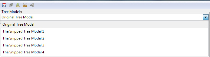
- As you snip one or more charts, the various versions of the chart will display in the Tree Models drop-down list.
- The Rules button displays the RpartRulesGUI.
- At any time, you can save a chart in one of the following formats: .pdf, .png, .jpg, .svg, or .wmf.
Decision-Tree Snipping
When working with a decision tree in a FancyPlot, you can edit it using the scissors icon. This enables you to determine which branches of the tree will be included in your decision tree.
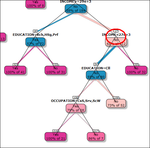
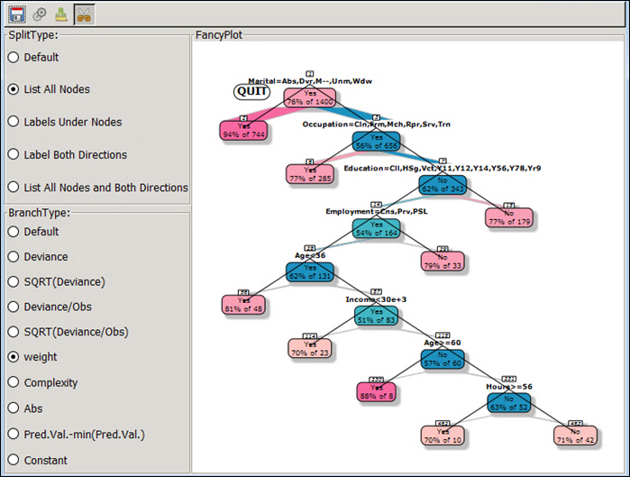
When snipping the decision tree, you must snip at the intersection of a branch, as shown in the red circle in the following image.
Once you have made a snip, you can click on the Quit icon to redraw the FancyPlot without the section that you just snipped. The Quit icon displays in the upper-left corner of the screen.
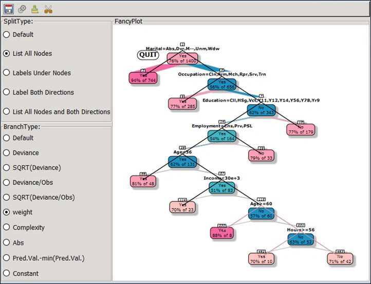
Within the decision tree, the lines of the branches are black until a snip is made. Snipping changes the color to grey, indicating that this portion of the decision tree will be removed based on your snip. This is shown in the following image.
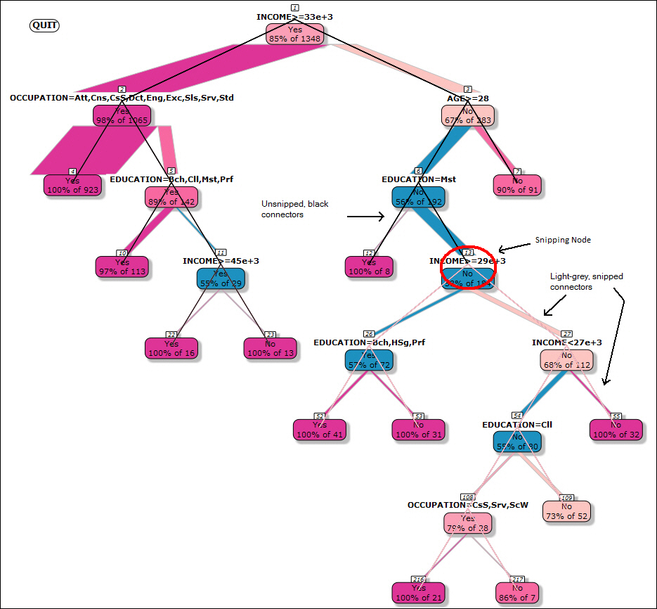
Note: If you snip at the top of the branch (where subordinate or lower branches are included), fewer nodes display, reducing the size of the chart (when the intersection and lower branches are removed).
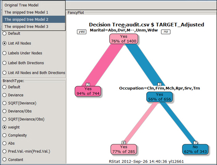
Once you click Quit, the updated FancyPlot displays (showing the area that was snipped).
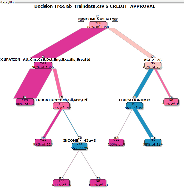
Note: In the diagram above, under the Education = Mst section, notice the node with YES = 100% of 8 before snipping and after snipping. The value of the No node is 58% of 184 after snipping, as well as before, however, this is now the end node.
As you are editing the decision tree, different versions of the tree are saved for each change you make, as shown in the following image.
This process creates a history for the chart with which you are working. You can create historical snapshots of your files and routines (PDFs or C Routines), as described in the following sections.
Saving a Decision Tree as a PDF File
|
How to: |
Each original and snipped tree model can be saved as a unique .pdf.
Procedure: How to Save a Decision Tree as a PDF File
- On the Model tab, select a model type from the Model Type list.
- Click Execute to review the model.
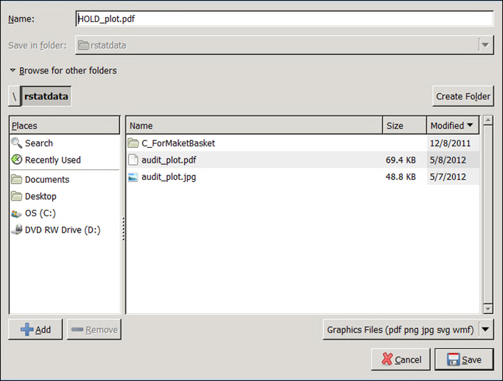
- Click Save to
save the current image to disk, as shown in the following image.
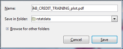
Note: You can specify a different name for the report in the Name field.
Saving a Decision Tree as a C Routine
|
How to: |
Each original and snipped tree model can be saved as a c routine.
Procedure: How to Export a Decision Tree as a C Routine
- On the Model tab, select a model type from the Model Type list.
- Click Execute to review the model.
- Click Export.
The Export C or PMML dialog box opens.
- Save the
file as a c routine, as shown in the following image.
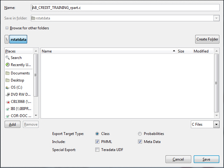
Note: You can specify a different name for the report in the Name field.
Creating FancyPlots
|
Reference: |
This section presents a series of screenshots that further illustrate the FancyPlot charting functionality. You can perform the following tasks with the FancyPlot GUI:
- Create a FancyPlot of a Decision Tree
- Snipping and resnipping of FancyPlots
- The ability to save the images you create
- Functionality in support of exporting to a C routine.
Reference: Create Different Types of Fancy Plots
The first screen shows a basic plotted chart, through which the current tree model can be exported. Using the SplitType and BranchType categories on the left, you can vary the output of your plot.
Note: Some combinations are not allowed. In those cases, an error message will display.
When working with a plotted chart, you can clear the chart from the user interface, leaving a blank canvas with which to work.
Once you have an output, you can save it to a file.
Next, you can then open the plot and use the edit (scissor image) to collapse the nodes in the tree.
Note: You will see a Quit icon in the left corner of the diagram. In addition, all nodes are connected by a solid black line.
When you click one of the nodes, the sub-tree will be colored.
Click Quit and another tree displays (without the selected sub--trees).
After each snipping procedure, the new tree model name is added to the drop-down list.
Select any portion of the new model (other than the original tree model) and perform a snip.
Select any model in the drop-down list and click Execute. The selected model will be drawn in the drawing area.
Note: It is recommended that you try at least three different models before making a determination.
Save the snipped tree and check the saved image.
| WebFOCUS | |
|
Feedback |