Explanation of the Regression Model
|
How to: |
|
Reference: |
What Is Regression Analysis?
Regression analysis is the method of using observations (data records) to quantify the relationship between a target variable (a field in the record set), also referred to as a dependent variable, and a set of independent variables, also referred to as a covariate. For example, regression analysis can be used to determine whether the dollar value of grocery shopping baskets (the target variable) is different for male and female shoppers (gender being the independent variable). The regression equation estimates a coefficient for each gender that corresponds to the difference in value.
The value of quantifying the relationship between a dependent variable and a set of independent variables is that the contribution of each independent variable to the value of the dependent variable becomes known. Once this is known, you need to know only the values of the independent variables in order to be able to make predictions about the value of the dependent variable. For example, when the coefficients for male and female shoppers are known, you can make precise revenue estimates for different distributions of shoppers. Specifically, you can predict the revenues for 80/20 females/males versus 60/40 females/males.
The goal of regression analysis is to generate the line that best fits the observations (the recorded data). The rationale for this is that the observations vary and thus will never fit precisely on a line. However, the best fitted line for the data leaves the least amount of unexplained variation, such as the dispersion of observed points around the line. Stated differently, a relationship that explains 90% of the variation in the observations is better than one that explains 75%. Conversely, a relationship with a better fit has a better predictive power.
How Does Linear Regression Work?
To illustrate how linear regression works, examine the relationship between the prices of vintage wines and the number of years since vintage. Each year, many vintage wine buyers gather in France and buy wines that will mature in 10 years. There are many stories and speculations on how the buyers determine the future prices of wine. Is the wine going to be good 10 years from now, and how much would it be worth? Imagine an application that could assist buyers in making those decisions by forecasting the expected future value of the wines. This is exactly what economists have done. They have collected data and created a regression model that estimates this future price. The current explanation of the regression is based on this model.
The provided sample data set contains 60 observations of prices for vintage wines that were sold at a wine auction. There are two columns, one for the price of each wine and another for the number of years since vintage. The data set, referred to as the training data set, is used to estimate the parameters in the equation.
The estimated equation can be used to predict wine prices when the year since vintage is known. In other words, it can be applied to another data set, referred to as the test data set, which contains only vintage years. Prices are derived by applying the equation to the vintage years in the training data set.
The following formula describes the linear relationship between price and years:
y = β0 + β1 x + error
- Dependent Variable Y. Y represents the price of each of the vintage wines observed in the auction.
- Independent Variable X. X is the time since vintage for each of the vintage wines observed in the auction. It is also referred to as a covariate.
- Parameters. β0 and β1 are parameters that are unknown and will be estimated by the equation. WebFOCUS RStat estimates these parameters when you run the regression model.
- Intercept. β0 is a constant that defines where the linear trend line intercepts the Y-axis.
- Coefficient. β1 is a constant that represents the rate of change in the dependent variable as a function of changes in the independent variable. It is the slope of the linear line, for example, it shows how prices increase with the increase in the number of vintage years, or how wines become more expensive the longer they mature. For other data sets, the trend can be the inverse, that is, the slope can be decreasing.
- Error. Represents the unexplained variation in the target variable. It is treated as a random variable that picks up all the variation in Y that is not explained by X.
The following image visually examines the nature of the relationship by plotting Y and X on a scatter plot with the trend line.
- All observations are plotted on the scatter plot.
- The linear trend illustrates the trend in the observed data.
- Variation shows the dispersion of the data points around the trend line.
- The ellipse shows the points that closely fit the line.
- The dashed square shows the observations that do not closely fit the line. These are referred to as outliers. Outliers are typically removed from the modeling data set. They can be filtered out. For example, the preceding scatter plot image above shows all points within the 1100 to 1700 price range as outliers. You can either filter out those outliers, or segment the data into different price ranges and build different regression models for each segment.
The following regression equation shows estimated parameters for the trend line:
y = -533 + 55 * x
To predict the price for a 15-year-old vintage wine, substitute x=15:
y = -533 + 55 * 15
y = -533 + 825
y = 292
How Does Multiple Linear Regression Work?
A simple linear equation rarely explains much of the variation in the data and for that reason, can be a poor predictor. In the case of vintage wine, time since vintage provides very little explanation for the prices of wines. The regression equation described in the simple linear regression section will poorly predict the future prices of vintage wines. Multiple linear regression enables you to add additional variables to improve the predictive power of the regression equation. On a very intuitive level, the producer of the wine matters. Thus, including the chateau as another independent variable is likely to increase the predictive power of the equation.
The following equation shows a multiple linear regression equation. The equation is conceptually similar to the simple regression equation, except for parameters β2 through βn, which represent the additional independent variables.
y = β0 + β1x1 + β2x2 + ... + βnxn + error
The independent variables in the vintage wine data set are:
- T (numeric variable). Is the average seasonal temperature in Celsius.
- WR (numeric variable). Is the winter rain from October to March.
- HR (numeric variable). Is the rain during the harvest season from August to September.
- TSV (numeric variable). Is the time since vintage, such as the number of years from the year in which the wine was produced until it was sold.
- Chateau (categorical variable). Is the name of the chateau in which the wine was produced.
The regression equation estimates a single parameter for the numeric variables and separate parameters for each unique value in the categorical variable. For example, there are six chateaus in the data set, and five coefficients. One chateau is used as a base against which all other chateaus are compared, and thus, no coefficient will be estimated for it. In other words, if prices have to be predicted for the reference chateau, 0 is entered in the equation.
The equation with the estimated parameters is:
Price = - 4744 + 1.03 * WR + 295.84 * T - 2.09 * HR + 8.06 * TSV + Chateau
The coefficients for each chateau are given in the output, as shown in the following image.
                         Estimate Std. Error t value   Pr(>|t|)
(Intercept)            -4743.7592  1027.7697  -4.616 0.00002762 ***
WRAIN                      1.0287     0.2513   4.093   0.000155 ***
DEGREES_IN_C             295.8356    58.8231   5.029 0.00000672 ***
HRAIN                     -2.0854     0.3686  -5.658 0.00000074 ***
TIME_SINCE_VINTAGE         8.0633    10.9301   0.738   0.464133
CHATEAUCos d'Estournel  -280.2000    99.3542  -2.820   0.006863 **
CHATEAULafite              7.8000    99.3542   0.079   0.937738
CHATEAULatour            177.9000    99.3542   1.791   0.079418 .
CHATEAUMontrose         -320.8000    99.3542  -3.229   0.002198 **
CHATEAUPichon Lalande   -228.4000    99.3542  -2.299   0.025730 *
---
Tip: The image below shows how the estimated parameter values are used as the coefficient values in the regression equation.
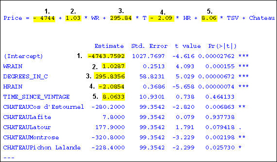
Note: Cheval Blanc is the reference chateau with a coefficient of 0. Therefore, it is not listed in the output. However, when scoring data, the predicted prices for the Cheval Blanc will be in the scoring output. For more information about the output, see Output From Linear Regression.
Vintage wine prices can be predicted by substituting the values for the independent variables, as in the simple regression equation used earlier.
A scoring application automatically generates the predicted prices, either for a single record or for a batch of records.
Practical Applications of Regression Analysis
Regression analysis is used for:
- Predictive Modeling. Regression is used most frequently for prediction. Credit scoring applications use input variables (data collected on the applicant) to predict the likelihood that the applicant will repay the loan. In budgeting and finance, regression is used to estimate the relationship between profit and cost, which later can be used in applications to generate what if scenarios.
- Segmentation. Regression is used to segment or to determine the lifetime value of customers. For example, a retailer may segment category purchases and baskets based on age groups and gender, thus creating a more targeted marketing campaign.
- Testing. Regression is used to evaluate the performance of marketing campaigns. It can test whether a campaign has increased the dollars spent in the test period compared to the prior period or whether certain age groups spend more than others, and so on.
Procedure: How to Create a Multiple Linear Regression (lm)
Note: The following example creates a multiple linear regression, using the wine_train data source, and targets PRICE_1991.
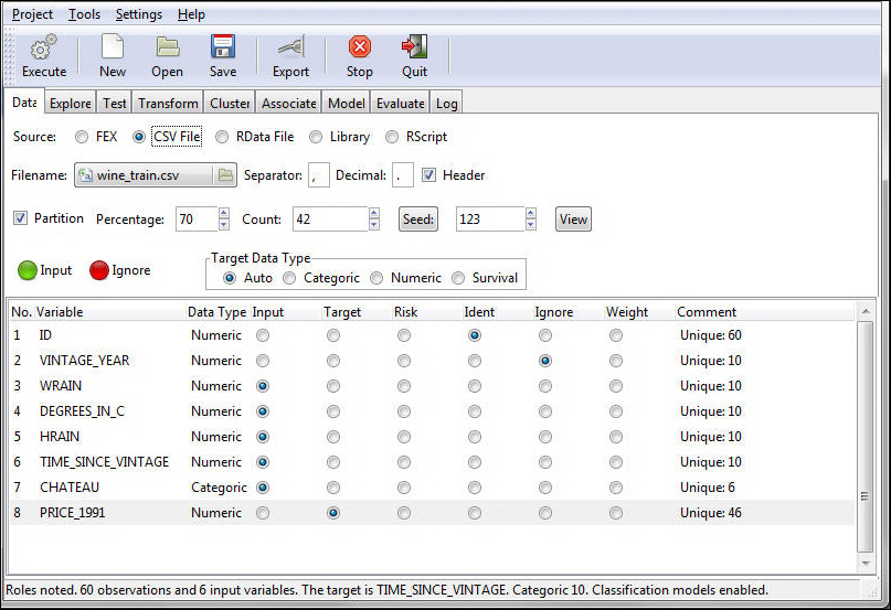
- Define the Model Data.
- Load the Wine data into RStat. For more information on loading data into RStat, see Getting Started With RStat.
- Select Ident for the ID variable.
- Select Ignore for the Vintage_Year variable.
- Select Target for the Price_1991 variable.
- Keep all the other variables as Input.
- Click Execute to set up the Model Data.
The status bar confirms your data settings, as shown in the following image.
- Select the Model tab to select the Model Data.
- Select Regression as the Type of model.
- Select Linear as
the Model Builder. This is the default option when Regression is
selected.
Note: Other available regression models are Generalized (Gaussian Regression model) and Poisson Regression models. Both models are built using Regression Generalized (glm).
- Click Execute to run the model.
The model data output appears in the bottom window of the Model tab, as shown in the following image.
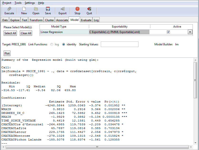
For details about the regression output, see Output From Linear Regression.
Reference: Output From Linear Regression
This section describes the linear regression output. Note that output may vary slightly due to sampling.
- Summary of the Regression model (built using lm). This
is the title of the summary provided for the model. It also specifies
which R function has been used to build the model. The model in
this case is built with the lm function.
Summary of the Regression model (built using lm):
- R Function Call. This
section shows the call to R and the data set or subset used in the
model. lm() indicates that we used the linear regression function
in R and c(3:8) indicates that columns 3 to 8 from the data set
were used in the model.
lm(formula = Price_1991 ~ ., data = crs$dataset[, c(3:8)])
- Residuals.
 Min       1Q   Median       3Q      Max
-404.62 -135.97   -9.47  95.58  4484.79
- Distribution of the Residuals. This
shows the distribution of the residuals. The residuals are the difference
between the prices in the training data set and the predicted prices
by this model. A negative residual is an overestimate and a positive
residual is an underestimate. Ideally, you should see a symmetrical
distribution with a median near zero. In this case, the median of
-9.47 is very close to zero.
Coefficients:
Coefficients: Estimate Std. Error t value Pr(>|t|) (Intercept) -5191.3914 1405.3794 -3.694 0.000820 *** WRAIN 0.9171 0.3502 2.619 0.013373 * Degrees_in_C 329.9655 83.0036 3.975 0.000375 *** HRAIN -1.8965 0.4753 -3.990 0.000360 *** Time_Since_Vintage 7.3211 13.6187 0.538 0.594587 ChateauCos d'Estournel -336.9234 130.7021 -2.578 0.014753 * ChateauLafite -70.7367 128.0801 -0.552 0.584590 ChateauLatour -27.4525 136.1005 -0.202 0.841422 ChateauMontrose -365.6623 140.1642 -2.609 0.013698 * ChateauPichon Lalande -283.3606 120.9652 -2.342 0.025538 * --- - Coefficient Name. Column 1 displays the names of the coefficients. Notice that for categorical variables, all values except the reference value are listed. For example, five out of six chateaus are listed. See How to Create a Multiple Linear Regression (lm).
- Estimate. These are the estimated values for the coefficients. Except for the reference chateau, notice the separate coefficient for each unique value of the categorical variable. The displayed coefficients are not standardized, for example, they are measured in their natural units, and thus cannot be compared with one another to determine which one is more influential in the model. Their natural units can be measured on different scales, as are temperature and rain.
- Standard Error. These are the standard errors of the coefficients. They can be used to construct the lower and upper bounds for the coefficient. An example is Coefficient ± Standard Error, which provides an indication where the value may fall if another sample data set is used. The standard error is also used to test whether the parameter is significantly different from 0. If a coefficient is significantly different from 0, then it has impact on the dependent variable (see t-value below).
- t-value. The t-value is the ratio of the regression coefficient β to its standard error (t = coefficient ÷ standard error). The t statistic tests the hypothesis that a population regression coefficient is 0. If a coefficient is different from zero, then it has a genuine effect on the dependent variable. However, a coefficient may be different from zero, but if the difference is due to random variation, then it has no impact on the dependent variable. In this example, Time_Since_Vintage is different from zero due to random variation and thus has no real impact on the dependent variable. The t-values are used to determine the P values (see below).
- Pr(>|t|). The P value indicates whether the independent variable has statistically significant predictive capability. It essentially shows the probability of the coefficient being attributed to random variation. The lower the probability, the more significant the impact of the coefficient. For example, there is less than a 1.3% chance that the WRAIN impact is due to random variation. The P value is automatically calculated by R by comparing the t-value against the Student's T distribution table. As a rule, a P value of less than 5% indicates significance. In theory, the P value for the constant could be used to determine whether the constant could be removed from the model.
- *. The asterisks in the last column indicate the significance ranking of the P values.
Signif. codes:
0 '***' 0.001 '**' 0.01 '*' 0.05 '.' 0.1 ' ' 1
The significance codes indicate how certain we can be that the coefficient has an impact on the dependent variable. For example, a significance level of 0.01 indicates that there is less than a 0.1% chance that the coefficient might be equal to 0 and thus be insignificant. Stated differently, we can be 99.9% sure that it is significant. The significance codes (shown by asterisks) are intended for quickly ranking the significance of each variable.
Residual standard error: 237.4 on 37 degrees of freedom.
Multiple R-squared: 0.7958
Adjusted R-squared: 0.7384
F-statistic: 13.86 on 9 and 32 DF, p-value: 0.000000009629.
- Residual Standard Error. This is the standard deviation of the error term in the regression equation (see Simple Regression, Error). The sample mean and the standard error can be used to construct the confidence interval for the mean. For example, it is the range of values within which the mean is expected to be if another representative data set is used.
- Degrees of Freedom (Df). This
column shows the degrees of freedom associated with the sources
of variance. The total variance has N -1 degrees of freedom. A data
set contains a number of observations - 60 in the vintage wine data set.
The cases are individual pieces of information that can be used
either to estimate parameters or variability. Each item (coefficient)
being estimated costs one degree of freedom; the rest are used to
estimate variability. For the vintage wine data set, you are estimating
nine coefficients. Therefore, there are 50 degrees of freedom for
the residuals.
For example, 50 = 60 - 1- 9.
- R-squared. R-squared is a measure of the proportion of variability explained by the regression. It is a number between zero and one, and a value close to zero suggests a poor model. In a multiple regression, each additional independent variable may increase the R-squared without improving the actual fit. An adjusted R-squared is calculated that represents the more accurate fit with multiple independent variables. The adjusted R-squared takes into account both the number of observations and the number of independent variables. It is always lower than R-squared.
- F-statistics and P-value. The
F-value, like the t-value (see t-value above), is calculated to
measure the overall quality of the regression.
The F-value is the Mean Square Regression divided by the Mean Square Residual. It is calculated on 9 Df for the coefficients and 50 Df for the residuals.
The P-value associated with this F-value is very small (5.596e-15). The P-value is a measure of how confident you can be that the independent variables reliably predict the dependent variable. P stands for probability and is usually interpreted as the probability that test data does not represent accurately the population from which it is drawn. If the P-value is 0.10, there is a 10% probability that the calculation for the test data is not true for the population. Conversely, you can be 90% certain that the results of the test data are true of the population.
For example, if the P-value were greater than 0.05, the group of independent variables does not show a statistically significant relationship with the dependent variable, or that the group of independent variables does not reliably predict the dependent variable. Note that this is an overall significance test assessing whether the group of independent variables when used together reliably predict the dependent variable, and does not address the ability of any of the particular independent variables to predict the dependent variable. The ability of each individual independent variable to predict the dependent variable is addressed in the coefficients table. (See P-values for the regression coefficients.)
Reference: Analysis of Variance (ANOVA) From Linear Regression
The following image shows the Model tab with the ANOVA table for the regression output. The ANOVA table provides statistics on each variable used in the regression equation.
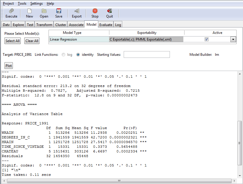
- Analysis of Variance Table. This is the title of this section.
- Response:
Price_1991.
                   Df  Sum Sq Mean Sq F value    Pr(>F)
WRAIN               1 2208522 2208522 44.7465 1.838e-08 ***
Degrees_in_C        1 4462834 4462834 90.4208 8.508e-13 ***
HRAIN               1 1702437 1702437 34.4928 3.445e-07 ***
Time_Since_Vintage  1   26861   26861  0.5442    0.4641
Chateau             5 1962422  392484  7.9521 1.422e-05 ***
Residuals          50 2467813   49356
---
- Variable Names. The first column shows the names of the variables used in the equation. It also lists the Error Term (Residuals).
- Df. The degrees of freedom taken by each variable. The numeric independent variables take 1 degree of freedom each. The categorical variable has six unique values but since one is set as a reference for which no estimate is generated, the variable Chateau takes only 5 degrees of freedom. 50 degrees of freedom are left for the residuals. For example, 50=60-9-1.
- Sum Sq and Mean Sq. The Sum of Squares and Mean Squares are computed so that you can compute the F statistics. (See next section on F-value.)
- F-value and P-value. The F-value is computed by dividing the Mean Square by the Mean Square Residual. For example, the F-value for WRAIN is calculated by dividing the Mean Squares for the variable (2,208,522) by the Mean Square for the Residuals (49,356). The compute F-Value is 44.7465. The F-value is used to compute the P-value which indicates whether a variable is significant or not in the over model (for further explanation on the F-value and the P-value, see F-statistics and P-value).
- Signif. codes:
0 '***' 0.001 '**' 0.01 '*' 0.05 '.' 0.1 ' ' 1
The significance codes indicate how certain we can be that the coefficient has an impact on the dependent variable. For example, a significance level of 0.001, indicates that there is less than a 0.1% chance that the coefficient might be equal to 0 and thus be insignificant. Stated differently, we can be 99% sure that it is significant. The significance codes (shown by asterisks) are intended for quickly ranking the significance of each variable.
- Time taken: 0.53
secs.
The time taken to generate the parameter estimates.
| WebFOCUS | |
|
Feedback |