Simplified Statistical Functions

Example: Calculating a Correlation

CORRELATION calculates the correlation between DOLLARS and BUDDOLLARS.

CORRELATION(DOLLARS, BUDDOLLARS)

For DOLLARS=46,156,290.00 and BUDDOLLARS=46,220,778.00, the result is 0.895691073.

Example: Partitioning Data Values Into Clusters

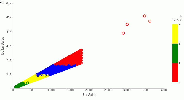
The following request partitions the DOLLARS field values into four clusters and displays the result as a scatter chart in which the color represents the cluster. The request uses the default values for the percent, iterations, and tolerance parameters by passing them as the value 0 (zero).

SET PARTITION_ON = PENULTIMATE
GRAPH FILE GGSALES
PRINT UNITS DOLLARS
COMPUTE KMEAN1/D20.2 TITLE 'K-MEANS'=  KMEANS_CLUSTER(4, AUTO, AUTO, AUTO, DOLLARS);
ON GRAPH SET LOOKGRAPH SCATTER
ON GRAPH PCHOLD FORMAT JSCHART
ON GRAPH SET STYLE *
INCLUDE=IBFS:/FILE/IBI_HTML_DIR/ibi_themes/Warm.sty,$
type = data, column = N2, bucket=y-axis,$
type=data, column= N1, bucket=x-axis,$
type=data, column=N3, bucket=color,$
GRID=OFF,$
*GRAPH_JS_FINAL
colorScale: {
		colorMode: 'discrete',
		colorBands: [{start: 1, stop: 1.99, color: 'red'}, {start: 2, stop: 2.99, color: 'green'}, 
               {start: 3, stop: 3.99, color: 'yellow'}, {start: 3.99, stop: 4, color: 'blue'} ]
	}
*END
ENDSTYLE
END

The output is shown in the following image.

Example: Calculating a Standard Deviation

STDDEV calculates the standard deviation of DOLLARS.

STDDEV(DOLLARS,S)

The result is 6,157.711080272.

Example: Creating a Multivariate Linear Regression Column

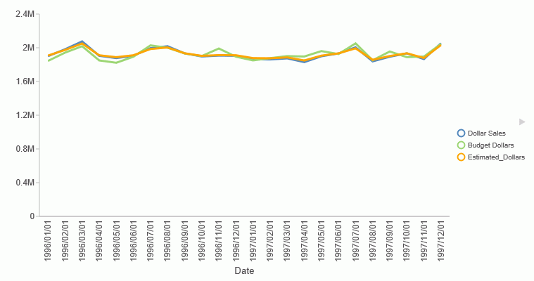
The following request uses the DOLLARS and BUDDOLLARS fields to generate a regression column named Estimated_Dollars.

GRAPH FILE GGSALES
SUM BUDUNITS UNITS BUDDOLLARS DOLLARS
COMPUTE Estimated_Dollars/F8 = MULTIREGRESS(DOLLARS, BUDDOLLARS);
BY DATE
ON GRAPH SET LOOKGRAPH LINE
ON GRAPH PCHOLD FORMAT JSCHART
ON GRAPH SET STYLE *
INCLUDE=IBFS:/FILE/IBI_HTML_DIR/ibi_themes/Warm.sty,$
type=data, column = n1, bucket = x-axis,$
type=data, column= dollars, bucket=y-axis,$
type=data, column= buddollars, bucket=y-axis,$
type=data, column= Estimated_Dollars, bucket=y-axis,$
*GRAPH_JS
"series":[
{"series":2, "color":"orange"}]
*END
ENDSTYLE
END

The output is shown in the following image. The orange line represents the regression equation.

Example: Using RESERVE to Run an R Script

The R script named wine_run_model.R predicts Bordeaux wine prices based on the average growing season temperature, the amount of rain during the harvest season, the amount of rain during the winter, and the age of the wine.

Using a configured connection (named MyRserve) for the Adapter for Rserve, and a sample data file named wine_input_sample.csv, you create the following synonym for the R script, as described in Statistics Adapters.

Master File

FILENAME=WINE_RUN_MODEL, SUFFIX=RSERVE  , $
  SEGMENT=INPUT_DATA, SEGTYPE=S0, $
    FIELDNAME=AGST, ALIAS=AGST, USAGE=D9.4, ACTUAL=STRING,
      MISSING=ON,
      TITLE='AGST', $
    FIELDNAME=HARVESTRAIN, ALIAS=HarvestRain, USAGE=I11, ACTUAL=STRING,
      MISSING=ON,
      TITLE='HarvestRain', $
    FIELDNAME=WINTERRAIN, ALIAS=WinterRain, USAGE=I11, ACTUAL=STRING,
      MISSING=ON,
      TITLE='WinterRain', $
    FIELDNAME=AGE, ALIAS=Age, USAGE=I11, ACTUAL=STRING,
      MISSING=ON,
      TITLE='Age', $
  SEGMENT=OUTPUT_DATA, SEGTYPE=U, PARENT=INPUT_DATA, $
    FIELDNAME=PRICE, ALIAS=Price, USAGE=D18.14, ACTUAL=STRING,
      MISSING=ON,
      TITLE='Price', $

Access File

SEGNAME=INPUT_DATA, 
  CONNECTION=MyRserve, 
  R_SCRIPT=/prediction/wine_run_model.r, 
  R_SCRIPT_LOCATION=WFRS, 
  R_INPUT_SAMPLE_DAT=prediction/wine_input_sample.csv, $

Now that the synonym has been created for the model, the model will be used to run against the following data file named wine_forecast.csv.

Year,Price,WinterRain,AGST,HarvestRain,Age,FrancePop
1952,7.495,600,17.1167,160,31,43183.569
1953,8.0393,690,16.7333,80,30,43495.03
1955,7.6858,502,17.15,130,28,44217.857
1957,6.9845,420,16.1333,110,26,45152.252
1958,6.7772,582,16.4167,187,25,45653.805
1959,8.0757,485,17.4833,187,24,46128.638
1960,6.5188,763,16.4167,290,23,46583.995
1961,8.4937,830,17.3333,38,22,47128.005
1962,7.388,697,16.3,52,21,48088.673
1963,6.7127,608,15.7167,155,20,48798.99
1964,7.3094,402,17.2667,96,19,49356.943
1965,6.2518,602,15.3667,267,18,49801.821
1966,7.7443,819,16.5333,86,17,50254.966
1967,6.8398,714,16.2333,118,16,50650.406
1968,6.2435,610,16.2,292,15,51034.413
1969,6.3459,575,16.55,244,14,51470.276
1970,7.5883,622,16.6667,89,13,51918.389
1971,7.1934,551,16.7667,112,12,52431.647
1972,6.2049,536,14.9833,158,11,52894.183
1973,6.6367,376,17.0667,123,10,53332.805
1974,6.2941,574,16.3,184,9,53689.61
1975,7.292,572,16.95,171,8,53955.042
1976,7.1211,418,17.65,247,7,54159.049
1977,6.2587,821,15.5833,87,6,54378.362
1978,7.186,763,15.8167,51,5,54602.193

The data file can be any type of file that R can read. In this case it is another .csv file. This file needs a synonym in order to be used in a report request. You create the synonym for this file using the Adapter for Delimited Files.

Following is the generated Master File, wine_forecast.mas.

FILENAME=WINE_FORECAST, SUFFIX=DFIX    , CODEPAGE=1252, 
   DATASET=prediction/wine_forecast.csv, $  
SEGMENT=WINE_FORECAST, SEGTYPE=S0, $
    FIELDNAME=YEAR1, ALIAS=Year, USAGE=I6, ACTUAL=A5V,
      MISSING=ON,      TITLE='Year', $
    FIELDNAME=PRICE, ALIAS=Price, USAGE=D8.4, ACTUAL=A7V,
      MISSING=ON,      TITLE='Price', $
    FIELDNAME=WINTERRAIN, ALIAS=WinterRain, USAGE=I5, ACTUAL=A3V,
      MISSING=ON,      TITLE='WinterRain', $
    FIELDNAME=AGST, ALIAS=AGST, USAGE=D9.4, ACTUAL=A8V,
      MISSING=ON,      TITLE='AGST', $
    FIELDNAME=HARVESTRAIN, ALIAS=HarvestRain, USAGE=I5, ACTUAL=A3V,
      MISSING=ON,      TITLE='HarvestRain', $
    FIELDNAME=AGE, ALIAS=Age, USAGE=I4, ACTUAL=A2V,      MISSING=ON,      TITLE='Age', $
    FIELDNAME=FRANCEPOP, ALIAS=FrancePop, USAGE=D11.3, ACTUAL=A11V,
      MISSING=ON,      TITLE='FrancePop', $

Following is the generated Access File, wine_forecast.acx.

SEGNAME=WINE_FORECAST,   DELIMITER=',',   ENCLOSURE=",   HEADER=YES,   CDN=COMMAS_DOT,   CONNECTION=<local>, $

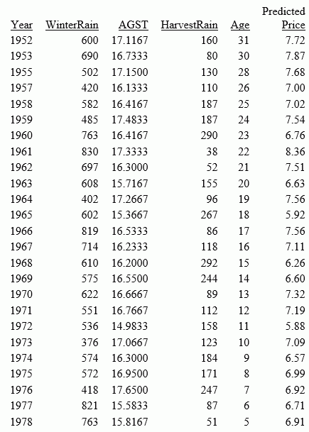
The following request, wine_forecast_price_report.fex, uses the RSERVE bulit-in function to run the script and return a report.

-*wine_forecast_price_report.fex
TABLE FILE PREDICTION/WINE_FORECAST
PRINT 
  YEAR
  WINTERRAIN
  AGST
  HARVESTRAIN
  AGE
     
  COMPUTE PREDICTED_PRICE/D18.2 MISSING ON ALL=
    RSERVE(prediction/wine_run_model, AGST, HARVESTRAIN, WINTERRAIN, AGE, Price);  AS 'Predicted,Price'

ON TABLE SET PAGE NOLEAD
ON TABLE SET STYLE *
GRID=OFF,$
ENDSTYLE 
END

The output is shown in the following image.