Reporting Language Enhancements
WebFOCUS is a complete information control system with comprehensive features for retrieving and analyzing data. It enables you to create reports quickly and easily. It also provides facilities for creating highly complex reports, but its strength lies in the simplicity of the request language. You can begin with simple queries and progress to complex reports as you learn about additional facilities.
Release 8.2.01 includes the Reporting Language new features available in Server Release 7707.
Additional Support for Alignment Grid
The HEADALIGN=BODY (Alignment Grid) feature has been expanded to support the following additional formats: PPTX and DHTML. The HEADALIGN=BODY feature enables you to insert a grid of cells in a heading to support more sophisticated styling.
For more information on the HEADALIGN=BODY feature, see the Creating Reports With WebFOCUS Language manual.
Defining Internal Borders in an Alignment Grid
The BORDERALL feature allows for the definition of internal borders within a HEADALIGN=BODY (Alignment Grid) element of a report.
The following example shows a DHTML request against the GGSALES data source. The request contains a subhead with HEADALIGN=BODY and BORDERALL=ON. The alignment grid in the subhead aligns with the data, and each item within the subhead is presented as fully bordered individual cells.
TABLE FILE GGSALES
SUM DOLLARS/D12CM AS '' UNITS/D12C AS ''
BY REGION PAGE-BREAK NOPRINT
BY CATEGORY AS ''
BY PRODUCT AS ''
ON REGION SUBHEAD
"<REGION <+0> &DATE <+0> "
"Category<+0>Product<+0>Dollars<+0>Units"
ON REGION SUBFOOT
""
ON TABLE PCHOLD FORMAT DHTML
WHERE REGION EQ 'West';
ON TABLE SET STYLE *
TYPE=REPORT, LEFTMARGIN=.75,RIGHTMARGIN=1,FONT=TAHOMA,SIZE=10,GRID=OFF,$
TYPE=SUBHEAD,HEADALIGN=BODY,BORDERALL=ON,$
TYPE=SUBHEAD,LINE=1,ITEM=3,COLSPAN=2, JUSTIFY=RIGHT, $
TYPE=SUBHEAD,LINE=2,STYLE=BOLD,$
END
The output is:
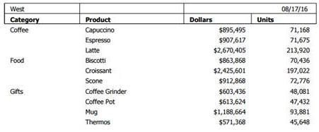
For more information on how the HEADALIGN=BODY and BORDERALL features work together, see the Creating Reports With WebFOCUS Language manual.
Enhancements to PPTX Output Format
|
Topics: |
The following are enhancements to the PPTX output format.
PNG Charts Embedded in Slides
The output image format for charts embedded in slides has been changed from JPG to PNG. PNG images are preferred as they produce better quality graph images, especially when displaying gradients, as well as provide support for transparency.
The PPTXGRAPHTYPE attribute enhances the quality of charts embedded into PowerPoint (PPTX) slides. As of Release 8.2.01M, you can use the PNG output format to enhance the image and text quality and support transparency.
This is useful for a number of important scenarios, including use of templates with background color and for overlapping a chart with other components and drawing objects.
The syntax is:
SET PPTXGRAPHTYPE={PNG|PNG_NOSCALE|JPEG}where:
- PNG
-
Scales the PNG image to twice its dimensions to get significantly improved quality. This may cause problems if you have non-scalable items in the chart, such as text with absolute point sizes (including embedded scales headings). The output file is also larger due to the larger bitmap. Text within the chart is noticeable sharper than the legacy JPEG format.
PNG preserves font sizes in the chart when it is internally rescaled for increased resolution. It converts absolute font sizes set in the stylesheet (*GRAPH_SCRIPT) to sizes expressed in virtual coordinates (which are relative to the dimensions of the chart) and generates font sizes for embedded headings and footings in virtual coordinates.
- PNG_NOSCALE
-
Renders in PNG, but does not scale. This produces slightly better quality than JPEG. Going from JPEG to PNG_NOSCALE makes the chart sharper, but has only a slight effect on the text.
- JPEG
-
Indicates legacy format. This is the default value.
For more information, see the Creating Reports With WebFOCUS Language manual.
PPTX Template Masters and Slide Layouts for Expanded Styling
A Microsoft PPTX template can contain one or more Slide Masters, defining a variety of different Slide Layouts. A Slide Master is the top slide in a hierarchy of slides that stores information about the theme and Slide Layouts of a presentation, including the background, color, fonts, effects, placeholder sizes, and positioning. You can incorporate two or more different styles or themes, such as backgrounds, color schemes, fonts, and effects, by inserting an individual Slide Master into the template for each different theme.
Note: Additional information on Microsoft PowerPoint Slide Layouts is available in an article titled What is a slide layout? on the Microsoft support site.
By default, the first Slide Layout in the first Slide Master is applied to slides on which WebFOCUS data is displayed.
With this new feature, WebFOCUS enables the developer to select any Slide Layout in any Slide Master in a PowerPoint template (POTX/POTM) or Presentation file (PPTX/PPTM). One Slide Layout may be applied to a slide or slides, displaying the output of a standard report, while one or different Slide Layouts may be applied to each Page Layout in a PPTX formatted Compound Document. The WebFOCUS generated output is placed on top of the styling on the selected Slide Layout.
For more information, see the Creating Reports With WebFOCUS Language manual.
Support for Page Size and Orientation
You can select the page size and orientation (Portrait or Landscape) for a PPTX formatted report, using the PAGESIZE and ORIENTATION style sheet attributes.
For more information, see the Creating Reports With WebFOCUS Language manual.
ReportCaster Bursting Support
Bursting PPTX formatted reports, including single reports and compound reports, is supported. Drill downs can be included in any of these burst reports.
For more information on ReportCaster bursting, see the ReportCaster manual.
Enhanced PDF Support for JPG Compression
|
How to: |
The compression algorithm used for JPG images embedded in PDF documents has been enhanced to generate considerably smaller PDF files, and to allow users to control elements of the JPEG compression method. The following new SET commands allow users to select the compression methodology (SET JPEGENCODE) and the image quality (SET JPEGQUALITY).
Syntax: How to Select the Compression Algorithm
SET JPEGENCODE = [FLATE|DCT]
where:
- FLATE
-
Fixed quality defined
Is a compression method, introduced in WebFOCUS Release 7.7 Version 03, which allows images within PDF files to be individually compressed. This method is the default for WebFOCUS Release 7.7 Version 03 through WebFOCUS Release 7.7 Version 06.
- DCT
-
Discrete Cosine Transform
Is a compression method, introduced in WebFOCUS Release 8.2 Version 01, which allows for the designation of the percentage of quality to retain. This method is the default in WebFOCUS Release 8.2 Version 01.
Note: In some images, quality loss is not noticeable when higher degrees of compression are applied. Generally, the higher the compression applied, the lower the image quality. Use SET JPEGQUALITY with the DCT setting to set the quality value.
Syntax: How to Select the Image Quality
SET JPEGQUALITY = n
where:
- n
-
Is the percentage of quality used with the DCT setting. This value can be from1-100. The default value is 100, where no quality is lost and minimal compression is applied.
Defining Hyperlink Colors
|
How to: |
You can use the HYPERLINK-COLOR attribute to designate a color for a hyperlink within a report. This applies to all hyperlinks generated in the report. You can define a single color for the entire report or different colors for each individual element.
Syntax: How to Set Hyperlink Colors
TYPE = type, HYPERLINK-COLOR = color
where:
- type
-
Is the report component you wish to affect. You can apply this keyword to the entire report using TYPE=REPORT. The attribute can also individually be set for any other element of the report.
- color
-
Can use any style sheet supported color value designation.
For more information, see the Creating Reports With WebFOCUS Language manual.
Automatically Resizing the Width of a Window or Frame With HFREEZE
In an HTML HFREEZE report, you can use the SET AUTOFIT command to automatically resize HTML report output to 100% of the current container width of the window or frame.
Enhanced Implementation of Peer Graphs
|
Topics: |
The following are enhancements to peer graphs.
HEX and RGB Color Designations
For HTML output format, in addition to named colors, you can now use hex and RGB for color designations in a StyleSheet.
The syntax is:
GRAPHCOLOR={color|RGB({r g b|#hexcolor}}
For more information, see the Creating Reports With WebFOCUS Language manual.
Setting a Color for Data Visualization Bar Graphs
For all output formats, you can use the GRAPHCOLORNEG StyleSheet attribute to set a color for the data visualization bar graphs that represent negative values.
The syntax is:
GRAPHNEGCOLOR={color|RGB({r g b|#hexcolor}}
For more information, see the Creating Reports With WebFOCUS Language manual.
SET FLOATMAPPING: Expanded Numeric Functionality
SET FLOATMAPPING enables you to take advantage of decimal-based precision numbers available in DB2 and Oracle, and extends that functionality to all numeric processing for floating point numbers. With this processing, you gain both precision, including improved rounding, and enhanced performance.
The syntax is
SET FLOATMAPPING = {D|M|X}where:
- D
-
Uses the standard double-precision processing. This is the default value.
- M
-
Uses a new internal format that provides decimal precision for double-precision floating point numbers up to 16 digits.
- X
-
Uses a new internal format that provides decimal precision for double-precision floating point numbers up to 34 digits.
Note: If the field is passed to a HOLD file, the internal data types X or M will be propagated to the USAGE and ACTUAL formats in the HOLD Master File.
New LOCALE Settings
|
Reference: |
New set parameters have been introduced to override locale-based attributes in a Master File.
These locale parameters can be accessed in the Web Console from the Workspace page, using the LOCALE button on the ribbon.
When set from this page, these parameter values are stored in the server global profile, edasprof.prf. You can also set them in a TABLE request, a FOCEXEC, or in any supported profile. Some of these parameters also have been implemented at the field level as display format options.
Note that the LANGUAGE parameter, which used to be stored in nlscfg.err, will also be saved in edasprof.prf.
Reference: Aliases for CDN Parameter Values
Aliases have been added to the existing CDN parameter values to make their meanings more clear. The following list describes the values from prior releases and the aliases that can now be used.
- OFF. Uses a dot (.) as the decimal separator and comma (,) as the thousands separator. The alias for OFF is COMMAS_DOT. This is the default value.
- ON. Uses a comma as the decimal separator and dot as the thousands separator. The alias for ON is DOTS_COMMA.
- SPACE. Uses a comma as the decimal separator and space as the thousands separator. The alias for SPACE is SPACES_COMMA.
- QUOTE. Uses a comma as the decimal separator and single quotation mark (') as the thousands separator. The alias for QUOTE is QUOTES_COMMA.
- QUOTEP. Uses a dot as the decimal separator and single quotation mark as the thousands separator. The alias for QUOTEP is QUOTES_DOT.
Reference: New Currency Locale Parameters and Display Options
The following SET parameters have been added for specifying locale-based currency display, when the :C currency display option is used. All other currency display options are unaffected by these settings.
CURRENCY_ISO_CODE
This parameter defines the ISO code for the currency symbol to use.
The syntax is:
SET CURRENCY_ISO_CODE = iso
where:
- iso
-
Is a standard three-character currency code such as USD for US dollars or JPY for Japanese yen. The default value is default, which uses the currency code for the configured language code.
CURRENCY_DISPLAY
This parameter defines the position of the currency symbol relative to the monetary number.
The syntax is:
SET CURRENCY_DISPLAY = pos
where:
- pos
-
Defines the position of the currency symbol relative to a number. The default value is default, which uses the position for the format and currency symbol in effect. Valid values are:
- LEFT_FIXED. The currency symbol is left-justified preceding the number.
- LEFT_FIXED_SPACE. The currency symbol is left-justified preceding the number, with at least one space between the symbol and the number.
- LEFT_FLOAT. The currency symbol precedes the number, with no space between them.
- LEFT_FLOAT_SPACE. The currency symbol precedes the number, with one space between them.
- TRAILING. The currency symbol follows the number, with no space between them.
- TRAILING_SPACE. The currency symbol follows the number, with one space between them.
CURRENCY_PRINT_ISO
This parameter defines what will happen when the currency symbol cannot be displayed by the code page in effect.
The syntax is:
SET CURRENCY_PRINT_ISO = {DEFAULT|ALWAYS|NEVER}where:
- DEFAULT
-
Replaces the currency symbol with its ISO code, when the symbol cannot be displayed by the code page in effect. This is the default value.
- ALWAYS
-
Always replaces the currency symbol with its ISO code.
- NEVER
-
Never replaces the currency symbol with its ISO code. If the currency symbol cannot be displayed by the code page in effect, it will not be printed at all.
Note: Using a Unicode environment allows the printing of all currency symbols, otherwise this setting is needed.
Currency Display Options
The CURRENCY_ISO_CODE, CURRENCY_DISPLAY, and CURRENCY_PRINT_ISO parameters can be applied on the field level as display parameters in a Master File DEFINE, a DEFINE command, or in a COMPUTE using the :C display option. The syntax is:
fld/fmt:C(CURRENCY_DISPLAY='pos',
   CURRENCY_ISO_CODE='iso',CURRENCY_PRINT_ISO='prt')= expression;
where:
- fld
-
Is the field to which the parameters are to be applied.
- fmt
-
Is a numeric format that supports a currency value.
- iso
-
Is a standard three-character currency code, such as USD for US dollars or JPY for Japanese yen. The default value is default, which uses the currency code for the configured language code.
- pos
-
Defines the position of the currency symbol relative to a number. The default value is default, which uses the position for the format and currency symbol in effect. Valid values are:
- LEFT_FIXED. The currency symbol is left-justified preceding the number.
- LEFT_FIXED_SPACE. The currency symbol is left-justified preceding the number, with at least one space between the symbol and the number.
- LEFT_FLOAT. The currency symbol precedes the number, with no space between them.
- LEFT_FLOAT_SPACE. The currency symbol precedes the number, with one space between them.
- TRAILING. The currency symbol follows the number, with no space between them.
- TRAILING_SPACE. The currency symbol follows the number, with one space between them.
- prt
-
Can be one of the following print options.
- DEFAULT
-
Replaces the currency symbol with its ISO code, when the symbol cannot be displayed by the code page in effect. This is the default value.
- ALWAYS
-
Always replaces the currency symbol with its ISO code.
- NEVER
-
Never replaces the currency symbol with its ISO code. If the currency symbol cannot be displayed by the code page in effect, it will not be printed at all.
- expression
-
Is the expression that creates the virtual field.
Note: If currency parameters are specified at multiple levels, the order of precedence is:
- Field level parameters.
- Parameters set in a request (ON TABLE SET).
- Parameters set in a FOCEXEC outside of a request.
- Parameters set in a profile, using the precedence for profile processing.
Example: Specifying Currency Parameters in a DEFINE
The following request creates a virtual field named Currency_parms that displays the currency symbol on the right using the ISO code for Japan, 'JPY'
DEFINE FILE WF_RETAIL_LITE
Currency_parms/D20.2:C(CURRENCY_DISPLAY='TRAILING',CURRENCY_ISO_CODE='JPY') = COGS_US;
END
TABLE FILE WF_RETAIL_LITE
SUM COGS_US Currency_parms
BY BUSINESS_REGION AS 'Region'
ON TABLE SET PAGE NOLEAD
ON TABLE SET STYLE *
GRID=OFF,$
END
The output is shown in the following image.
Reference: New Date and Time Locale Parameters
The following SET parameters have been added to specify the order of date components, the date separator character, and the time separator character for the &TOD system variable.
DATE_ORDER
This parameter defines the order of date components for display. The syntax is:
SET DATE_ORDER = {DEFAULT|DMY|MDY|YMD}where:
- DEFAULT
-
Respects the original order of date components. This is the default value.
- DMY
-
Displays all dates in day/month/year order.
- MDY
-
Displays all dates in month/day/year order.
- YMD
-
Displays all dates in year/month/day order.
DATE_SEPARATOR
This parameter defines the separator for date components for display.
The syntax is:
SET DATE_SEPARATOR = separator
where:
- separator
-
Can be one of the following values.
- DEFAULT, which respects the separator defined by the USAGE format of the field.
- SLASH, which uses a slash (/) to separate date components.
- DASH, which uses a dash (-) to separate date components.
- BLANK, which uses a blank to separate date components.
- DOT, which uses a dot (.) to separate date components.
- NONE, which does not separate date components.
TIME_SEPARATOR
This parameter defines the separator for time components for the &TOD system variable.
The syntax is:
SET TIME_SEPARATOR = {DOT|COLON}where:
- DOT
-
Uses a dot (.) to separate time components. This is the default value.
- COLON
-
Uses a colon (:) to separate time components.
Reference: Usage Notes for Locale-Based Date and Time Parameters
- DATE_ORDER and DATE_SEPARATOR override the specified date order for all date and date-time displays unless they include a translation display option (T, Tr, t, or tr), in which case the specified order is produced. To limit the scope to a request, use the ON TABLE SET phrase.
- To use these settings with the Dialogue Manager system variables, (for example, &DATE, &TOD, &YMD, &DATEfmt, and &DATXfmt) append the suffix .DATE_LOCALE to the system variable. This allows system variables that are localized to coexist with non-localized system variables.
Example: Setting Date and Time Parameters for System Variables
The following applies the DATE_ORDER and DATE_SEPARATOR parameters to the &DATE system variable.
SET DATE_SEPARATOR = DASH
SET DATE_ORDER = DMY
-TYPE NON-LOCALIZED: &DATE
-TYPE LOCALIZED: &DATE.DATE_LOCALE
The output is:
NON-LOCALIZED: 04/07/17
LOCALIZED: 07-04-17
Applying Selection Criteria to the Internal Matrix Prior to COMPUTE Processing
|
How to: |
|
Reference: |
WHERE TOTAL tests are applied to the rows of the internal matrix after COMPUTE calculations are processed in the output phase of the report. WHERE_GROUPED tests are applied to the internal matrix values prior to COMPUTE calculations. The processing then continues with COMPUTE calculations, and then WHERE TOTAL tests. This allows the developer to control the evaluation, and is particularly useful in recursive calculations.
Syntax: How to Apply WHERE_GROUPED Selection Criteria
WHERE_GROUPED expression
where:
- expression
-
Is an expression that does not refer to more than one row in the internal matrix. For example, it cannot use the LAST operator to refer to or retrieve a value from a prior record.
Example: Using a WHERE_GROUPED Test
The following request has two COMPUTE commands. The first COMPUTE checks to see if the business region value has changed, incrementing a counter if it has. This allows us to sequence the records in the matrix. The second COMPUTE creates a rolling total of the days delayed within the business region.
TABLE FILE WF_RETAIL_LITE
SUM  DAYSDELAYED AS DAYS
COMPUTE CTR/I3 = IF BUSINESS_REGION EQ LAST BUSINESS_REGION THEN CTR+1 ELSE 1;
COMPUTE NEWDAYS = IF BUSINESS_REGION EQ LAST BUSINESS_REGION THEN NEWDAYS+DAYSDELAYED ELSE DAYSDELAYED;
BY BUSINESS_REGION AS Region
BY TIME_MTH
WHERE BUSINESS_REGION NE 'Oceania'
ON TABLE SET PAGE NOPAGE
END
The output is shown in the following image.
The following version of the request adds a WHERE TOTAL test to select only those months where DAYSDELAYED exceeded 200 days..
TABLE FILE WF_RETAIL_LITE
SUM  DAYSDELAYED AS DAYS
COMPUTE CTR/I3 = IF BUSINESS_REGION EQ LAST BUSINESS_REGION THEN CTR+1 ELSE 1;
COMPUTE NEWDAYS= IF BUSINESS_REGION EQ LAST BUSINESS_REGION THEN NEWDAYS+DAYSDELAYED ELSE DAYSDELAYED;
BY BUSINESS_REGION AS Region
BY TIME_MTH
WHERE BUSINESS_REGION NE 'Oceania'
WHERE TOTAL DAYSDELAYED GT 200
ON TABLE SET PAGE NOPAGE
END
The output is shown in the following image. The COMPUTE calculations for CTR and NEWDAYS was processed prior to eliminating the rows in which TOTAL DAYSDELAYED were 200 or less, so their values are the same as in the original output. This does not correctly reflect the sequence of records and the rolling total of the values that are actually displayed on the output. To do this, we need to select the appropriate months (DAYSDELAYED GT 200) before the COMPUTE expressions are evaluated. This requires WHERE_GROUPED.
The following version of the request replaces the WHERE TOTAL test with a WHERE_GROUPED test.
TABLE FILE WF_RETAIL_LITE
SUM  DAYSDELAYED AS DAYS
COMPUTE CTR/I3 = IF BUSINESS_REGION EQ LAST BUSINESS_REGION THEN CTR+1 ELSE 1;
COMPUTE NEWDAYS= IF BUSINESS_REGION EQ LAST BUSINESS_REGION THEN NEWDAYS+DAYSDELAYED ELSE DAYSDELAYED;
BY BUSINESS_REGION AS Region
BY TIME_MTH
WHERE BUSINESS_REGION NE 'Oceania'
WHERE_GROUPED DAYSDELAYED GT 200
ON TABLE SET PAGE NOPAGE
END
The output is shown in the following image. The COMPUTE calculation for NEWDAYS was processed after eliminating the rows in which TOTAL DAYSDELAYED were 200 or less, so its values are based on fewer rows than the calculations in the original request. This is verified by the CTR values, which are now in a continuous sequence. The rolling total now reflects the values that are actually displayed on the report output.
Reference: Usage Notes for WHERE_GROUPED
- If the expression refers to multiple rows in the internal matrix,
the following message is generated and processing stops.
(FOC32692) WHERE_GROUPED CANNOT REFER TO OTHER LINES OF REPORT
- A COMPUTE that does not reference multiple lines will be evaluated prior to WHERE_GROUPED tests, and may, therefore, be used in an expression and evaluated as part of a WHERE_GROUPED test.
- WHERE_GROUPED can be optimized for SQL data sources by creating a GROUP BY fieldname HAVING expression clause, where the expression is the WHERE_GROUPED selection criteria.
PARTITION_AGGR: Creating Rolling Calculations
|
How to: |
|
Reference: |
Using the PARTITION_AGGR function, you can generate rolling calculations based on a block of rows from the internal matrix of a TABLE request. In order to specify how to determine the limits of the rolling calculations, you specify a partition of the data based on either a sort field or the entire TABLE. Within either type of break, you can start calculating from the beginning of the break or a number of rows prior to the current row. You can stop the rolling calculation at the current row or the end of the partition.
By default, the field values used in the calculations are the summed values of a measure in the request. Certain prefix operators can be used to add a column to the internal matrix and use that column in the rolling calculations. The rolling calculation can be SUM, AVE, CNT, MIN, MAX, FST, or LST.
Syntax: How to Generate Rolling Calculations Using PARTITION_AGGR
PARTITION_AGGR([prefix.]measure,{sortfield|TABLE},from,to,operation)where:
- prefix.
-
Defines an aggregation operator to apply to the measure before using it in the rolling calculation. Valid operators are:
- SUM. which calculates the sum of the measure field values. SUM is the default operator.
- CNT. which calculates a count of the measure field values.
- AVE. which calculates the average of the measure field values.
- MIN. which calculates the minimum of the measure field values.
- MAX. which calculates the maximum of the measure field values.
- FST. which retrieves the first value of the measure field.
- LST. which retrieves the last value of the measure field.
Note: The operators PCT., RPCT., TOT., MDN., and DST. are not supported. COMPUTEs that reference those unsupported operators are also not supported.
- measure
-
Is the measure field to be aggregated. It can be a real field in the request or a calculated value generated with the COMPUTE command, as long as the COMPUTE does not reference an unsupported prefix operator.
- sortfield
-
Is a BY or ACROSS field that defines the boundary of the partition. Operations will not cross a boundary. In the request the BY HIGHEST phrase to sort high-to-low is supported. ACROSS COLUMNS AND is also supported, but BY ROWS OVER and FOR are not supported.
Specifying TABLE as the boundary makes the partition boundary the entire internal matrix.
For example, if the sort is BY YEAR BY MONTH, with data from both 2014 and 2015, specifying the boundary as YEAR means that January 2015 - 2 will be valued as zero (0) or MISSING, as two months prior to January 2015 would cross the YEAR boundary. However, specifying TABLE as the boundary and requesting - 2 months would return the data for November 2014.
- from
-
Identifies the starting point for the rolling calculation. Valid values are:
- -n, which starts the calculation n rows back from the current row.
- B, which starts the calculation at the beginning of the current sort break (the first line with the same sort field value as the current line).
- to
-
Identifies the ending point of the rolling calculation. Valid values are:
- C, which ends the rolling calculation at the current row in the internal matrix.
- E, which ends the rolling calculation at the end of the sort break (the last line with the same sort value as the current row.)
- operation
-
Specifies the rolling calculation used on the values in the internal matrix. Supported operations are:
- SUM. which calculates a rolling sum.
- AVE. which calculates a rolling average.
- CNT. which counts the rows in the partition.
- MIN. which returns the minimum value in the partition.
- MAX, which returns the maximum value in the partition.
- FST. which returns the first value in the partition.
- LST. which returns the last value in the partition.
The calculation is performed prior to any WHERE TOTAL tests, but after WHERE_GROUPED tests.
Example: Calculating a Rolling Average
The following request calculates a rolling average of the current line and the previous line in the internal matrix within the quarter.
TABLE FILE WF_RETAIL_LITE
SUM COGS_US
COMPUTE AVE1/D12.2M = PARTITION_AGGR(COGS_US, TIME_QTR, -1, C, AVE);
BY BUSINESS_REGION
BY TIME_QTR
BY TIME_MTH
WHERE BUSINESS_REGION EQ 'North America' OR 'South America'
ON TABLE SET PAGE NOLEAD
END
The output is shown in the following image. Within each quarter, the first average is just the value from Q1, as going back 1 would cross a boundary. The second average is calculated using the first two rows within that quarter, and the third average is calculated using rows 2 and 3 within the quarter.
The following changes the rolling average to start from the beginning of the sort break.
COMPUTE AVE1/D12.2M = PARTITION_AGGR(COGS_US, TIME_QTR ,B, C, AVE);
The output is shown in the following image. Within each quarter, the first average is just the value from Q1, as going back would cross a boundary. The second average is calculated using the first two rows within that quarter, and the third average is calculated using rows 1 through 3 within the quarter.

The following command uses the partition boundary TABLE.
COMPUTE AVE1/D12.2M = PARTITION_AGGR(COGS_US, TABLE, B, C, AVE);
The output is shown in the following image. The rolling average keeps adding the next row to the average until a break in the business region sort field.
Reference: Usage Notes for PARTITION_AGGR
- Fields referenced in the PARTITION_AGGR parameters but not previously mentioned in the request, will not be counted in column notation or propagated to HOLD files.
- Using the WITHIN phrase for a sum is the same as computing PARTITION_AGGR
on the WITHIN sort field from B (beginning of sort break) to E (end
of sort break) using SUM, as in the following example.
TABLE FILE WF_RETAIL_LITE
SUM COGS_US WITHIN TIME_QTR AS 'WITHIN Qtr'
COMPUTE PART_WITHIN_QTR/D12.2M = PARTITION_AGGR(COGS_US, TIME_QTR, B, E, SUM);
BY BUSINESS_REGION AS Region
BY TIME_QTR
BY TIME_MTH
WHERE BUSINESS_REGION EQ 'North America' OR 'South America'
ON TABLE SET PAGE NOPAGE
END
The output is shown in the following image.
With other types of calculations, the results are not the same. For example, the following request calculates the average within quarter using the WITHIN phrase and the average with quarter using PARTITION_AGGR.
TABLE FILE WF_RETAIL_LITE
SUM  COGS_US AS Cost
CNT.COGS_US AS Count AVE.COGS_US WITHIN TIME_QTR AS 'Ave Within'
COMPUTE PART_WITHIN_QTR/D12.2M = PARTITION_AGGR(COGS_US, TIME_QTR, B, E, AVE);
BY BUSINESS_REGION AS Region
BY TIME_QTR
ON TIME_QTR SUBTOTAL COGS_US CNT.COGS_US
BY TIME_MTH
WHERE BUSINESS_REGION EQ 'North America'
ON TABLE SET PAGE NOPAGE
END
The output is shown in the following image. The average using the WITHIN phrase divides the total cost for the quarter by the total count of instances for the quarter (for example, $435,992.00/1514 =$287.97), while PARTITION_AGGR divides the total cost for the quarter by the number of report rows in the quarter (for example, $435,992.00/3 = $145,330.67).
- If you use PARTITION_AGGR to perform operations for specific time periods using an offset, for example, an operation on the quarters for different years, you must make sure that every quarter is represented. If some quarters are missing for some years, the offset will not access the correct data. In this case, generate a HOLD file that has every quarter represented for every year (you can use BY QUARTER ROWS OVER 1 OVER 2 OVER 3 OVER 4) and use PARTITION_AGGR on the HOLD file.
PARTITION_REF: Using Prior Field Values in Calculations
|
How to: |
|
Reference: |
Use of LAST in a calculation retrieves the LAST value of the specified field the last time this calculation was performed. The PARTITION_REF function enables you to specify both how many rows back to go in order to retrieve a prior value, and a sort break within which the prior value calculation will be contained.
Syntax: How to Retrieve Prior Field Values for Use in a Calculation
PARTITION_REF([prefix.]field, {sortfield|TABLE}, -offset)where:
- prefix
-
Is optional. If used, it can be one of the following aggregation operators:
- AVE. Average
- MAX. Maximum
- MIN. Minimum
- CNT. Count
- SUM. Sum
- field
-
Is the field whose prior value is to be retrieved.
- {srtfield|TABLE}
-
Is the sort break within which to go back to retrieve the value. TABLE means retrieve the value without regard to sort breaks. Operations will not cross a partition boundary.
The Sort field may use BY HIGHEST to indicate a HIGH-TO-LOW sort. ACROSS COLUMNS AND is supported. BY ROWS OVER and FOR are not supported.
- -offset
-
Is the integer number of records back to go to retrieve the value.
If the offset is prior to the partition boundary sort value, the return will be the default value for the field. The calculation is performed prior to any WHERE TOTAL tests, but after WHERE_GROUPED tests.
Example: Retrieving a Previous Record With PARTITION_REF
The following request retrieves the previous record within the sort field PRODUCT_CATEGORY.
TABLE FILE WF_RETAIL_LITE
SUM DAYSDELAYED
COMPUTE NEWDAYS/I5=PARTITION_REF(DAYSDELAYED, PRODUCT_CATEGORY, -1);
BY PRODUCT_CATEGORY
BY PRODUCT_SUBCATEG
ON TABLE SET PAGE NOPAGE
END
The output is shown in the following image. The first value within each sort break is zero because there is no prior record to retrieve.
The following request retrieves the average cost of goods from two records prior to the current record within the PRODUCT_CATEGORY sort field.
TABLE FILE WF_RETAIL_LITE
SUM COGS_US AVE.COGS_US AS Average
COMPUTE PartitionAve/D12.2M=PARTITION_REF(AVE.COGS_US, PRODUCT_CATEGORY, -2);
BY PRODUCT_CATEGORY
BY PRODUCT_SUBCATEG
ON TABLE SET PAGE NOPAGE
END
The output is shown in the following image.
Replacing the function call with the following syntax changes the partition boundary to TABLE.
COMPUTE PartitionAve/D12.2M=PARTITION_REF(AVE.COGS_US, TABLE, -2);
The output is shown in the following image.
Reference: Usage Notes for PARTITION_REF
- Fields referenced in the PARTITION_REF parameters but not previously mentioned in the request, will not be counted in column notation or propagated to HOLD files.
Increased Number of ACROSS Columns in a Report
The limit on the number of ACROSS columns has been removed. The total number of sort fields (BY and ACROSS) still has a maximum of 128.
Increased Number of Verb Objects in a TABLE Request
The number of verb objects supported in a TABLE request is unlimited. However, errors can occur if the output is being sent to a format that has a limit on the number of columns, if the system has a maximum record length that cannot contain the number of columns of output, or if the amount of memory needed to store the output is unavailable.
Specifying a Geographic Role in a DEFINE or COMPUTE
|
How to: |
If you define a virtual field or create a calculated value that is location-related, you can specify a geographic role. This may be helpful when using the field in a location-based chart request.
Syntax: How to Specify a Geographic Role in a DEFINE or COMPUTE
DEFINE name/fmt (GEOGRAPHIC_ROLE = georole)
   [MISSING ON NEEDS {SOME|ALL} DATA] = expression;
COMPUTE name/fmt (GEOGRAPHIC_ROLE = georole)
[MISSING ON NEEDS {SOME|ALL} DATA] = expression;where:
- name
-
Is a name for the virtual field or calculated value.
- fmt
-
Is a valid format specification for the geographic value.
- georole
-
Is a valid geographic role. Geographic roles can be names, postal codes, ISO (International Organization for Standardization) codes, FIPS (Federal Information Processing Standards) codes, or NUTS (Nomenclature of Territorial Units for Statistics ) codes. The following is a list of supported geographic roles.
- ADDRESS_FULL. Full address.
- ADDRESS_LINE. Number and street name.
- CITY. City name.
- CONTINENT. Continent name.
- CONTINENT_ISO2. Continent ISO-3166 code.
- COUNTRY. Country name.
- COUNTRY_FIPS. Country FIPS code.
- COUNTRY_ISO2. Country ISO-3166-2 code
- COUNTRY_ISO3. Country ISO-3166-3 code
- GEOMETRY_AREA. Geometry area.
- GEOMETRY_LINE. Geometry line.
- GEOMETRY_POINT. Geometry point.
- LATITUDE. Latitude.
- LONGITUDE. Longitude.
- NUTS0. Country name (NUTS level 0).
- NUTS0_CC. Country code (NUTS level 0).
- NUTS1. Region name (NUTS level 1).
- NUTS1_CC. Region code (NUTS level1).
- NUTS2. Province name (NUTS level 2).
- NUTS2_CC. Province code (NUTS level 2).
- NUTS3. District name (NUTS level 3).
- NUTS3_CC. District code (NUTS level 3).
- POSTAL_CODE. Postal code.
- STATE. State name.
- STATE_FIPS. State FIPS code.
- STATE_ISO_SUB. US State ISO subdivision code.
- USSCITY. US city name.
- USCITY_FIPS. US city FIPS code.
- USCOUNTY. US county name.
- USCOUNTY_FIPS. US county FIPS code.
- USSTATE. US state name.
- USSTATE_ABBR. US state abbreviation.
- USSTATE_FIPS. US state FIPS code.
- ZIP3. US 3-digit postal code.
- ZIP5. US 5-digit postal code.
Example: Specifying a Geographic Role in a DEFINE
The following defines a field whose geographic role is the state name.
DEFINE FILE WF_RETAIL_LITE
STATENAME/A20 (GEOGRAPHIC_ROLE = STATE) = STATE_PROV_NAME;
END
Limiting the Number of Stacked Commands and Loop Iterations
|
How to: |
As WebFOCUS commands are encountered in a procedure, they are placed on a stack in memory (called FOCSTACK). The procedure is executed and the stack counter reset to zero (0) as a result a -RUN command, certain system variables, or the end of the procedure.
The parameter DMH_STACKLIM sets the maximum number of lines allowed in the FOCSTACK. This parameter is designed to prevent runaway tasks that generate a FOCSTACK that uses an inordinate amount of memory.
If users are not careful in designing loops in Dialogue Manager, they can inadvertently cause an infinite looping condition.
The parameter DMH_LOOPLIM sets the maximum number of Dialogue Manager loop iterations allowed, using -REPEAT or -GOTO commands.
DMH_STACKLIM and DMH_LOOPLIM should be set high enough to run your existing reports and procedures without error for your entire session. It is recommended that if you set these parameters, you should set them in a profile.
Syntax: How to Limit the Number of Stacked Commands
SET DMH_STACKLIM = n
where:
- n
-
Sets the maximum number of lines allowed in FOCSTACK. The default value is zero (0), which does not limit the number of stacked commands.
Syntax: How to Limit the Number of Loop Iterations
SET DMH_LOOPLIM = n
where:
- n
-
Sets the maximum number of loop iterations allowed. The default value is zero (0), which does not limit the number of loop iterations.
New Report-Level Prefix Operators
|
How to: |
|
Reference: |
Prefix operators have been added for headings, footings, subheadings, subfootings, verb objects, and calculated values (COMPUTEs) that calculate the average, maximum, minimum, and count for the entire report. They are based on the TOT. operator, which calculates total values to include in a heading.
These operators cannot be referenced in WHERE or WHERE TOTAL tests. However, they can be used in a COMPUTE command to generate a calculated value that can be used in a WHERE TOTAL test.
Syntax: How to Calculate Report-Level Average, Maximum, Minimum, and Count Values
operator.field
where:
- operator
-
Can be one of the following prefix operators.
- TOTAVE. Calculates the average value of the field for the entire table.
- TOTMAX. Calculates the maximum value of the field for the entire table.
- TOTMIN. Calculates the minimum value of the field for the entire table.
- TOTCNT. Calculates the count of the field instances for the entire table.
- field
-
Is a verb object or calculated value in the request.
Example: Using Prefix Operators in a Heading
The following request uses prefix operators in the heading.
TABLE FILE WF_RETAIL_LITE
HEADING
"Heading Calculations:"
"Total:      <TOT.COGS_US"
"Count:                   <TOTCNT.COGS_US"
"Average:           <TOTAVE.COGS_US"
"Minimum:            <TOTMIN.COGS_US"
"Maximum:      <TOTMAX.COGS_US"
SUM COGS_US CNT.COGS_US AS Count AVE.COGS_US AS Average
MIN.COGS_US AS Minimum MAX.COGS_US AS Maximum
BY BUSINESS_REGION AS Region
BY PRODUCT_CATEGORY AS Category
WHERE BUSINESS_REGION NE 'Oceania'
ON TABLE SUBTOTAL COGS_US CNT.COGS_US  AS Total
ON TABLE SET PAGE NOPAGE
ON TABLE SET SHOWBLANKS ON
ON TABLE SET STYLE *
type=report,grid=off, size=11,$
ENDSTYLE
END
The output is shown in the following image.
Reference: Usage Notes for Report-Level Prefix Operators
- These operators can be used on a field in a heading or footing without being referenced in a display command in the request.
- They work in a heading or footing for real or virtual (DEFINE) fields. They work in a display command field list on real fields, virtual (DEFINE) fields, and calculated (COMPUTE) values that are calculated prior to their use in the request.
- They can be used in subheadings and subfootings to reference the total value for the entire report.
Controlling Processing of Delimited Files
The SET PCOMMA=DFIX command causes delimited files with SUFFIX=COM, COMT, TAB, and TABT to be processed through the Adapter for DFIX. This processing provides more complete and meaningful messages and some changes to the processing of missing values when two delimiters in a row are encountered. With DFIX processing, a missing value is assigned to the field.
In order to be eligible for DFIX processing, the delimited file must satisfy the following requirements.
- Each record must be completely contained on one line and
terminated with the crlf (carriage return/line feed) character combination.
If a break is found within a record, the following message displays.
(FOC229) ERROR READING EXTERNAL DATA FILE: file
- The ENCLOSURE can be only in the first position after the delimiter for COM (new) and COMT records. Otherwise, it will not be recognized.
- The number of fields on a line cannot exceed the number of fields
defined in the Master File. If there are more, the following message
displays.
(FOC416) MORE VALUES SUPPLIED THAN FIELDS IN THE MASTER FILE DESCRIPTION
Format Display Option for Percentage Calculation
|
How to: |
The lowercase p display option converts a number to a percent by multiplying it by 100. It then displays the number followed by a percent symbol (%). This is different from the % format option, which does not calculate a percent, it just displays a percent symbol after the number.
Note: This option is not supported for output formats XLSX and EXL2K.
Syntax: How to Display a Percentage
field/floatfmtp
where:
- field
-
Is a numeric field.
- floatfmt
-
Is a numeric format of type F or D.
Example: Displaying a Percentage Using Display Option p
The following request displays the PCT_INC field (which is a decimal value) and redisplays it as a percentage:
TABLE FILE EMPLOYEE
PRINT PCT_INC PCT_INC/F10p
END
The output is:
  PCT_INC      PCT_INC
  -------      -------
      .10          10%
      .12          12%
      .10          10%
      .04           4%
      .00           0%
      .05           5%
      .00           0%
      .00           0%
      .10          10%
      .00           0%
      .00           0%
      .15          15%
      .00           0%
      .07           7%
      .00           0%
      .04           4%
      .00           0%
      .05           5%
      .00           0%
Start of Week Parameter for the DTRUNC Function
Given a date or date-time value and a time period, the DTRUNC function returns the date that is the beginning of that period. The parameter WEEK has been added, which returns the date that represents the first date of the given week. By default, the first day will be Sunday, but this can be changed using the WEEKFIRST parameter.
Example: Using the Start of Week Parameter for DTRUNC
The following request returns the date that is the start of the week for the start date of certain employees:
DEFINE FILE WF_RETAIL
DAY1/WT = DTRUNC(START_DATE, DAY);
WKSTART/YYMD = DTRUNC(START_DATE, WEEK);
DAY2/WT = DTRUNC(WKSTART, DAY);
END
TABLE FILE WF_RETAIL
PRINT START_DATE
DAY1 AS 'DOW 1'
WKSTART AS 'Start,of Week'
DAY2 AS 'DOW 2'
BY EMPLOYEE_NUMBER
WHERE START_DATE GT '20130101'
WHERE EMPLOYEE_NUMBER CONTAINS 'AH'
ON TABLE SET PAGE NOPAGE
END
The output is:
  Employee      Start              Start
  Number        Date        DOW 1  of Week     DOW 2
  --------      -----       -----  -------     -----
  AH118         2013/01/15  TUE    2013/01/13  SUN
  AH2272        2013/01/17  THU    2013/01/13  SUN
  AH288         2013/11/11  MON    2013/11/10  SUN
  AH3520        2013/09/23  MON    2013/09/22  SUN
  AH3591        2013/09/22  SUN    2013/09/22  SUN
  AH5177        2013/07/21  SUN    2013/07/21  SUN
Function DTRUNC Returns the Last Day of a Calendar Period
Given a date or timestamp and a component, DTRUNC returned the first date within the period specified by that component.
The following components have been added that return the last date within the period specified by the component.
- YEAR_END
- QUARTER_END
- MONTH_END
- WEEK_END
This function is available in both WebFOCUS and SQL.
The calculators in the Synonym Editor and Data Flow show the new parameter values.
Note: You can change which day is considered the first day of the week using the WEEKFIRST parameter. By default, it is Sunday.
Example: Returning the Date of the First and Last Days of a Week
The following request returns the dates that corresponds to the first day of the week and the last day of the week for the given date.
DEFINE FILE WF_RETAIL
WEEKSTART/YYMD = DTRUNC(START_DATE, WEEK);
WEEKEND/YYMD = DTRUNC(START_DATE, WEEK_END);
END
TABLE FILE WF_RETAIL
PRINT START_DATE WEEKSTART AS 'Start,of Week'
WEEKEND AS 'End,of Week'
BY EMPLOYEE_NUMBER
WHERE EMPLOYEE_NUMBER CONTAINS 'AH1'
ON TABLE SET PAGE NOPAGE
END
The output is shown in the following image.
Simplified Numeric Functions
|
Topics: |
New numeric functions have been developed that make it easier to understand and enter the required arguments. These functions have streamlined parameter lists, similar to those used by SQL functions. In some cases, these simplified functions provide slightly different functionality than previous versions of similar functions.
The simplified functions do not have an output argument. Each function returns a value that has a specific data type.
When used in a request against a relational data source, these functions are optimized (passed to the RDBMS for processing).
Note:
- The simplified numeric functions are supported in Dialogue Manager.
- The simplified numeric functions are not supported in WebFOCUS Maintain.
CEILING: Returning the Smallest Integer Value Greater Than or Equal to a Value
|
How to: |
CEILING returns the smallest integer value that is greater than or equal to a number.
Syntax: How to Return the Smallest Integer Greater Than or Equal to a Number
CEILING(number)
where:
- number
-
Numeric
Is the number whose ceiling will be returned. The output data type is the same as the input data type.
Example: Returning the Ceiling of a Number
In the following request, CEILING returns the smallest integer greater than or equal to the GROSS_PROFIT_US value.
DEFINE FILE WF_RETAIL_LITE
CEIL1/D7.2= CEILING(GROSS_PROFIT_US);
END
TABLE FILE WF_RETAIL_LITE
PRINT GROSS_PROFIT_US/D9.2  CEIL1
ON TABLE SET PAGE NOPAGE
END
The partial output follows. Note that even though the value returned is an integer, it is returned with the same format as the CEIL1 field (D7.2):
  Gross Profit     CEIL1
  ------------     -----
        165.00    165.00
         13.99     14.00
         60.99     61.00
        225.98    226.00
         79.99     80.00
         44.59     45.00
         94.30     95.00
        238.50    239.00
        199.99    200.00
         68.99     69.00
         63.58     64.00
        129.99    130.00
         37.49     38.00
         75.99     76.00
         13.99     14.00
        119.00    119.00
        -30.01    -30.00
         54.99     55.00
        189.98    190.00
         44.59     45.00
         91.98     92.00
         89.00     89.00
         59.50     60.00
        129.99    130.00
         54.00     54.00
        109.98    110.00
         98.99     99.00
         98.99     99.00
         99.99    100.00
         44.59     45.00
EXPONENT: Raising e to a Power
|
How to: |
EXPONENT raises the constant e to a power.
Syntax: How to Raise the Constant e to a Power
EXPONENT(power)
where:
- power
-
Numeric
Is the power to which to raise e. The output data type is numeric.
Example: Raising e to a Power
The following request prints the value of e and the value of e raised to the fifth power.
DEFINE FILE WF_RETAIL_LITE
EXP1/D12.5 = EXPONENT(1);
EXP2/D12.5 = EXPONENT(5);
END
TABLE FILE WF_RETAIL_LITE
PRINT EXP1 EXP2
BY BUSINESS_REGION AS Region
WHERE BUSINESS_REGION EQ 'EMEA'
WHERE RECORDLIMIT EQ 1
ON TABLE SET PAGE NOPAGE
END
The output is shown in the following image.
FLOOR: Returning the Largest Integer Less Than or Equal to a Value
|
How to: |
FLOOR returns the largest integer value that is less than or equal to a number.
Syntax: How to Return the Largest Integer Less Than or Equal to a Number
FLOOR(number)
where:
- number
-
Numeric
Is the number whose floor will be returned. The output data type is the same as the input data type.
Example: Returning the Floor of a Number
In the following request, FLOOR returns the largest integer less than or equal to the GROSS_PROFIT_US value.
DEFINE FILE WF_RETAIL_LITE
FLOOR1/D7.2= FLOOR(GROSS_PROFIT_US);
END
TABLE FILE WF_RETAIL_LITE
PRINT GROSS_PROFIT_US/D9.2  FLOOR1
ON TABLE SET PAGE NOPAGE
END
Partial output follows. Note that even though the value returned is an integer, it is returned with the same format as the FLOOR1 field (D7.2):
  Gross Profit    FLOOR1
  ------------    ------
        165.00    165.00
         13.99     13.00
         60.99     60.00
        225.98    225.00
         79.99     79.00
         44.59     44.00
         94.30     94.00
        238.50    238.00
        199.99    199.00
         68.99     68.00
         63.58     63.00
        129.99    129.00
         37.49     37.00
         75.99     75.00
         13.99     13.00
        119.00    119.00
        -30.01    -31.00
         54.99     54.00
        189.98    189.00
         44.59     44.00
         91.98     91.00
         89.00     89.00
         59.50     59.00
        129.99    129.00
         54.00     54.00
        109.98    109.00
         98.99     98.00
         98.99     98.00
         99.99     99.00
         44.59     44.00
MOD: Calculating the Remainder From a Division
|
How to: |
MOD calculates the remainder from a division. The output data type is the same as the input data type.
Syntax: How to Calculate the Remainder From a Division
MOD(dividend, divisor)
where:
- dividend
-
Numeric
Is the value to divide.
- divisor
-
Numeric
Is the value to divide by.
If the divisor is zero (0), the dividend is returned.
Example: Calculating the Remainder From a Division
In the following request, MOD returns the remainder of PRICE_DOLLARS divided by DAYSDELAYED:
DEFINE FILE WF_RETAIL_LITE
MOD1/D7.2= MOD(PRICE_DOLLARS, DAYSDELAYED);
END
TABLE FILE WF_RETAIL_LITE
PRINT PRICE_DOLLARS/D7.2  DAYSDELAYED/I5 MOD1
WHERE DAYSDELAYED GT 1
ON TABLE SET PAGE NOPAGE
ON TABLE PCHOLD FORMAT WP
END
Partial output follows:
Price    Days
   Dollars  Delayed      MOD1
   -------  -------      ----
    399.00        3       .00
    489.99        3       .99
    786.50        2       .50
    599.99        4      3.99
     29.99        4      1.99
    169.00        2      1.00
    219.99        2      1.99
    280.00        3      1.00
     79.99        4      3.99
    145.99        2      1.99
    399.99        3       .99
    349.99        3      1.99
    169.00        3      1.00
POWER: Raising a Value to a Power
|
How to: |
POWER raises a base value to a power.
Syntax: How to Raise a Value to a Power
POWER(base, power)
where:
- base
-
Numeric
Is the value to raise to a power. The output value has the same data type as the base value. If the base value is integer, negative power values will result in truncation.
- power
-
Numeric
Is the power to which to raise the base value.
Example: Raising a Base Value to a Power
In the following request, POWER returns the value COGS_US/20.00 raised to the power stored in DAYSDELAYED:
DEFINE FILE WF_RETAIL_LITE
BASE=COGS_US/20.00;
POWER1= POWER(COGS_US/20.00,DAYSDELAYED);
END
TABLE FILE WF_RETAIL_LITE
PRINT BASE IN 15 DAYSDELAYED POWER1
BY PRODUCT_CATEGORY
WHERE PRODUCT_CATEGORY EQ 'Computers'
WHERE DAYSDELAYED NE 0
ON TABLE SET PAGE NOPAGE
END
Partial output follows:
  Product                              Days
  Category                BASE         Delayed          POWER1
  --------                ----         -------          ------
  Computers              12.15               3        1,793.61
                         16.70               2          278.89
                          8.35               1            8.35
                          8.10               2           65.61
                          4.05               1            4.05
                          4.05               2           16.40
                          4.05               4          269.04
                          8.35               1            8.35
                         16.70               1           16.70
                          8.35               3          582.18
                          8.35               1            8.35
                          4.05               1            4.05
                          4.05               1            4.05
                          8.35               4        4,861.23
                          8.35              -1             .12
                          8.35               1            8.35
                          8.35               3          582.18
Simplified Character Functions
|
Topics: |
New simplified character functions CONCAT, REGEX, REPLACE, and SPLIT functions have been added.
LAST_NONBLANK: Retrieving the Last Field Value That is Neither Blank nor Missing
|
How to: |
LAST_NONBLANK retrieves the last field value that is neither blank nor missing. If all previous values are either blank or missing, LAST_NONBLANK returns a missing value.
Syntax: How to Return the Last Value That is Neither Blank nor Missing
LAST_NONBLANK(field)
where:
- field
-
Is the field name whose last non-blank value is to be retrieved. If the current value is not blank or missing, the current value is returned.
Note: LAST_NONBLANK cannot be used in a compound expression, for example, as part of an IF condition.
Example: Retrieving the Last Non-Blank Value
The following request shows the SALARY field, the LAST_NONBLANK value from a DEFINE, and the LAST_NONBLANK value from a COMPUTE.
DEFINE FILE EMPLOYEE
MYSAL/I5 MISSING ON=IF DEPARTMENT EQ 'MIS' THEN SALARY ELSE MISSING;
LAST_NONBLANK1/I5 MISSING ON= LAST_NONBLANK(MYSAL);
END
TABLE FILE EMPLOYEE
PRINT LAST_NAME MYSAL  LAST_NONBLANK1
COMPUTE LAST_NONBLANK2/I5 MISSING ON=LAST_NONBLANK(MYSAL);
ON TABLE SET PAGE NOLEAD
ON TABLE SET STYLE *
GRID=OFF,$
END
The output is shown in the following image.
REGEX: Matching a String to a Regular Expression
|
How to: |
The REGEX function matches a string to a regular expression and returns true (1) if it matches and false (0) if it does not match.
A regular expression is a sequence of special characters and literal characters that you can combine to form a search pattern.
Many references for regular expressions exist on the web.
For a basic summary, see the section Summary of Regular Expressions in Chapter 2, Security, of the Server Administration manual.
Syntax: How to Match a String to a Regular Expression
REGEX(string, regular_expression)
where:
- string
-
Alphanumeric
Is the character string to match.
- regular_expression
-
Alphanumeric
Is a regular expression enclosed in single quotation marks (') constructed using literals and metacharacters. The following metacharacters are supported
- . represents any single character
- * represents zero or more occurrences
- + represents one or more occurrences
- ? represents zero or one occurrence
- ^ represents beginning of line
- $ represents end of line
- [] represents any one character in the set listed within the brackets
- [^] represents any one character not in the set listed within the brackets
- | represents the Or operator
- \ is the Escape Special Character
- () contains a character sequence
For example, the regular expression '^Ste(v|ph)en$' matches values starting with Ste followed by either ph or v, and ending with en.
Note: The output value is numeric.
Example: Matching a String Against a Regular Expression
The following request matches the FIRSTNAME field against the regular expression '^Sara(h?)$', which matches Sara or Sarah:
TABLE FILE WF_RETAIL_LITE
PRINT FIRSTNAME AND COMPUTE
REG1/I1=REGEX(FIRSTNAME,'^Sara(h?)$') ;
BY LASTNAME/A10
WHERE LASTNAME EQ 'Allen'
END
The output is
              First
  LASTNAME    Name                  REG1
  --------    -----                 ----
  Allen       Penny                    0
              Rosemary                 0
              Amber                    0
              Julie                    0
              Sarah                    1
              Leo                      0
              Margret                  0
              Donna                    0
              Damian                   0
              Alexander                0
              Diego                    0
              Amber                    0
              Susan                    0
              Amber                    0
              Sara                     1
              Sara                     1
CONCAT: Concatenating Strings After Removing Trailing Blanks From the First
|
How to: |
CONCAT removes trailing blanks from a string and then concatenates another string to it. The output is returned as variable length alphanumeric.
Syntax: How to Concatenate Strings After Removing Trailing Blanks From the First
CONCAT(string1, string2)
where:
- string2
-
Alphanumeric
Is a string whose trailing blanks will be removed.
- string1
-
Alphanumeric
Is a string whose leading and trailing blanks will be preserved.
Example: Concatenating Strings After Removing Blanks From the First
The following request concatenates city names with state names. Note that the city and state names are converted to fixed length alphanumeric fields before concatenation.
DEFINE FILE WF_RETAIL_LITE
CITY/A50 = CITY_NAME;
STATE/A50 = STATE_PROV_NAME;
CONCAT_CS/A100 = CONCAT(CITY,STATE);
END

TABLE FILE WF_RETAIL_LITE
SUM CITY AS City STATE AS State CONCAT_CS AS Concatenation
BY STATE_PROV_NAME NOPRINT
WHERE COUNTRY_NAME EQ 'United States'
WHERE STATE LE 'Louisiana'
ON TABLE SET PAGE NOLEAD
END
The output is shown in the following image.
REPLACE: Replacing a String
|
How to: |
REPLACE replaces all instances of a search string in an input string with the given replacement string. The output is always variable length alphanumeric with a length determined by the input parameters.
Syntax: How to Replace all Instances of a String
REPLACE(input_string , search_string , replacement)
where:
- input_string
-
Alphanumeric or text (An, AnV, TX)
Is the input string.
- search_string
-
Alphanumeric or text (An, AnV, TX)
Is the string to search for within the input string.
- replacement
-
Alphanumeric or text (An, AnV, TX)
Is the replacement string to be substituted for the search string. It can be a null string ('').
Example: Replacing a String
REPLACE replaces the string 'South' in the Country Name with the string 'S.'
SET TRACEUSER = ON
SET TRACEON = STMTRACE//CLIENT
SET TRACESTAMP=OFF
DEFINE FILE WF_RETAIL_LITE
NEWNAME/A20 = REPLACE(COUNTRY_NAME, 'SOUTH', 'S.');
END
TABLE FILE WF_RETAIL_LITE
SUM COUNTRY_NAME
BY NEWNAME AS 'New,Name'
WHERE COUNTRY_NAME LIKE 'S%'
ON TABLE SET PAGE NOLEAD
END
The generated SQL passes the REPLACE function to the DBMS REPLACE function.
SELECT
REPLACE(T3."COUNTRY_NAME",'SOUTH','S.'),
MAX(T3."COUNTRY_NAME")
FROM
wrd_wf_retail_geography T3
WHERE
(T3."COUNTRY_NAME" LIKE 'S%')
GROUP BY
REPLACE(T3."COUNTRY_NAME",'SOUTH','S.')
ORDER BY
REPLACE(T3."COUNTRY_NAME",'SOUTH','S.');
The output is shown in the following image.
Example: Replacing All Instances of a String
In the following request, the virtual field DAYNAME1 is the string DAY1 with all instances of the string 'DAY' replaced with the string 'day'. The virtual field DAYNAME2 has all instances of the string 'DAY' removed.
DEFINE FILE WF_RETAIL
DAY1/A30 = 'SUNDAY MONDAY TUESDAY';
DAYNAME1/A30 = REPLACE(DAY1, 'DAY', 'day' );
DAYNAME2/A30 = REPLACE(DAY1, 'DAY', '' );
END
TABLE FILE WF_RETAIL
PRINT DAY1 OVER
DAYNAME1 OVER
DAYNAME2
WHERE EMPLOYEE_NUMBER EQ 'AH118'
ON TABLE SET PAGE NOPAGE
END
The output is:
  DAY1      SUNDAY MONDAY TUESDAY
  DAYNAME1  SUNday MONday TUESday
  DAYNAME2  SUN MON TUES
SPLIT: Extracting an Element From a String
|
How to: |
The SPLIT function returns a specific type of element from a string. The output is returned as variable length alphanumeric.
Syntax: How to Extract an Element From a String
SPLIT(element, string)
where:
- element
-
Can be one of the following keywords:
- EMAIL_DOMAIN. Is the domain name portion of an email address in the string.
- EMAIL_USERID. Is the user ID portion of an email address in the string.
- URL_PROTOCOL. Is the URL protocol in the string.
- URL_HOST. Is the host name of the URL in the string.
- URL_PORT. Is the port number of the URL in the string.
- URL_PATH. Is the URL path in the string.
- NAME_FIRST. Is the first token (group of characters) in the string. Tokens are delimited by blanks.
- NAME_LAST. Is the last token (group of characters) in the string. Tokens are delimited by blanks.
- string
-
Alphanumeric
Is the string from which the element will be extracted.
Example: Extracting an Element From a String
The following request defines strings and extracts elements from them.
DEFINE FILE WF_RETAIL_LITE
STRING1/A50 WITH COUNTRY_NAME= 'http://www.informationbuilders.com';
STRING2/A20 = 'user1@ibi.com';
STRING3/A20 = 'Louisa May Alcott';
Protocol/A20 = SPLIT(URL_PROTOCOL, STRING1);
Path/A50 = SPLIT(URL_PATH, STRING1);
Domain/A20 = SPLIT(EMAIL_DOMAIN, STRING2);
User/A20 =  SPLIT(EMAIL_USERID, STRING2);
First/A10 = SPLIT(NAME_FIRST, STRING3);
Last/A10 = SPLIT(NAME_LAST, STRING3);
END
TABLE FILE WF_RETAIL_LITE
SUM Protocol Path User Domain First Last
ON TABLE SET PAGE NOLEAD
END
The output is shown in the following image.
CHECKMD5: Computing an MD5 Hash Check Value
|
How to: |
CHECKMD5 takes an alphanumeric input value and returns a 128-bit value in a fixed length alphanumeric string, using the MD5 hash function. A hash function is any function that can be used to map data of arbitrary size to data of fixed size. The values returned by a hash function are called hash values. They can be used for assuring the integrity of transmitted data.
Syntax: How to Compute an MD5 Hash Check Value
CHECKMD5(buffer)
where:
- buffer
-
Is a data buffer whose hash value is to be calculated. It can be a set of data of different types presented as a single field, or a group field in one of the following data type formats: An, AnV, or TXn.
Example: Calculating an MD5 Hash Check Value
The following request calculates an MD5 hash check value and converts it to an alphanumeric hexadecimal value for display.
DEFINE FILE WF_RETAIL_LITE
MD5/A32 = HEXTYPE(CHECKMD5(PRODUCT_CATEGORY));
END
TABLE FILE WF_RETAIL_LITE
SUM MD5
BY PRODUCT_CATEGORY
ON TABLE SET PAGE NOLEAD
ON TABLE SET STYLE *
TYPE=REPORT,FONT=COURIER,$
 ENDSTYLE
END
The output is shown in the following image. The monospaced font shows that although the input values have varying length, the output has a fixed length.
CHECKSUM: Computing a Hash Sum
|
How to: |
CHECKSUM computes a hash sum, called the checksum, of its input parameter, as a whole number in format I11. This can be used for equality search of the fields. A checksum is a hash sum used to ensure the integrity of a file after it has been transmitted from one storage device to another.
Syntax: How to Compute a CHECKSUM Hash Value
CHECKSUM(buffer)
where:
- buffer
-
Is a data buffer whose hash index is to be calculated. It can be a set of data of different types presented as a single field, in one of the following data type formats: An, AnV, or TXn.
Example: Calculating a CHECKSUM Hash Value
The following request computes a checksum hash value.
DEFINE FILE WF_RETAIL_LITE
CHKSUM/I11 = (CHECKSUM(PRODUCT_CATEGORY));
END
TABLE FILE WF_RETAIL_LITE
PRINT CHKSUM
BY PRODUCT_CATEGORY
WHERE PRODUCT_CATEGORY NE LAST PRODUCT_CATEGORY
ON TABLE SET PAGE NOLEAD
END
The output is shown in the following image.
Simplified Conversion Functions
New simplified conversion functions CHAR, CTRL_CHAR, EDIT2, HEXTYPE, TO_INTEGER, and TO_NUMBER have been added.
CHAR: Returning a Character Based on a Numeric Code
|
How to: |
The CHAR function accepts a decimal integer and returns the character identified by that number converted to ASCII or EBCDIC, depending on the operating environment. The output is returned as variable length alphanumeric. If the number is above the range of valid characters, a null is returned.
Syntax: How to Return a Character Based on a Numeric Code
CHAR(number_code)
where:
- number_code
-
Integer
Is a field, number, or numeric expression whose whole absolute value will be used as a number code to retrieve an output character.
For example, a TAB character is returned by CHAR(9) in ASCII environments, or by CHAR(5) in EBCDIC environments.
Example: Using the CHAR Function to Insert Control Characters Into a String
The following request defines a field with carriage return (CHAR(13)) and line feed (CHAR(10)) characters inserted between the words HELLO and GOODBYE (in an ASCII environment). To show that these characters were inserted, the output is generated in PDF format and the StyleSheet attribute LINEBREAK='CRLF' is used to have these characters respected and print the field value on two lines.
DEFINE FILE WF_RETAIL_LITE
MYFIELD/A20 WITH COUNTRY_NAME='HELLO' | CHAR(13) | CHAR(10) | 'GOODBYE';
END
TABLE FILE WF_RETAIL_LITE
SUM MYFIELD
ON TABLE PCHOLD FORMAT PDF
ON TABLE SET PAGE NOLEAD
ON TABLE SET STYLE *
TYPE=REPORT,LINEBREAK='CRLF',$
ENDSTYLE
END
The output is shown in the following image.

CTRLCHAR: Returning a Non-Printable Control Character
|
How to: |
The CTRLCHAR function returns a nonprintable control character specific to the running operating environment, based on a supported list of keywords. The output is returned as variable length alphanumeric.
Syntax: How to Return a Non-Printable Control Character
CTRLCHAR(ctrl_char)
where:
- ctrl_char
-
Is one of the following keywords.
- NUL returns a null character.
- SOH returns a start of heading character.
- STX returns a start of text character.
- ETX returns an end of text character.
- EOT returns an end of transmission character.
- ENQ returns an enquiry character.
- ACK returns an acknowledge character.
- BEL returns a bell or beep character.
- BS returns a backspace character.
- TAB or HT returns a horizontal tab character.
- LF returns a line feed character.
- VT returns a vertical tab character.
- FF returns a form feed (top of page) character.
- CR returns a carriage control character.
- SO returns a shift out character.
- SI returns a shift in character.
- DLE returns a data link escape character.
- DC1 or XON returns a device control 1 character.
- DC2 returns a device control 2 character.
- DC3 or XOFF returns a device control 3 character.
- DC4 returns a device control 4 character.
- NAK returns a negative acknowledge character.
- SYN returns a synchronous idle character.
- ETB returns an end of transmission block character.
- CAN returns a cancel character.
- EM returns an end of medium character.
- SUB returns a substitute character.
- ESC returns an escape, prefix, or altmode character.
- FS returns a file separator character.
- GS returns a group separator character.
- RS returns a record separator character.
- US returns a unit separator character.
- DEL returns a delete, rubout, or interrupt character.
Example: Using the CTRLCHAR Function to Insert Control Characters Into a String
The following request defines a field with carriage return (CTRLCHAR(CR)) and line feed (CTRLCHAR(LF)) characters inserted between the words HELLO and GOODBYE. To show that these characters were inserted, the output is generated in PDF format and the StyleSheet attribute LINEBREAK='CRLF' is used to have these characters respected and print the field value on two lines.
DEFINE FILE WF_RETAIL_LITE
MYFIELD/A20 WITH COUNTRY_NAME='HELLO' | CTRLCHAR(CR) | CTRLCHAR(LF) | 'GOODBYE';
END
TABLE FILE WF_RETAIL_LITE
SUM MYFIELD
ON TABLE PCHOLD FORMAT PDF
ON TABLE SET PAGE NOLEAD
ON TABLE SET STYLE *
TYPE=REPORT,LINEBREAK='CRLF',$
ENDSTYLE
END
The output is shown in the following image.

EDIT2: Converting a Numeric, Date, or Date-Time Value to a Character String
|
How to: |
The EDIT2 function converts a numeric, date, or date-time value to a character string based on a specified format. The format must be valid for the data supplied. The output is returned as variable length alphanumeric.
Syntax: How to Convert a Numeric, Date, or Date_Time Value to a Character String
EDIT2(in_value, 'format')
where:
- in_value
-
Numeric, date, or date-time
Is any numeric value or a date in either standard date or date-time format. If the date is given in standard date format, all of its time components are assumed to be zero.
- 'format'
-
Is a numeric, date, or date-time format enclosed in single quotation marks (').
Example: Converting a Date to a Character String
The following request defines a date field as YYMD format and converts it to a character string (CharDate) in YYMtrD format.
DEFINE FILE WF_RETAIL_LITE
DATE1/YYMD = TIME_DATE_DAY_COMPONENT;
CharDate/A20 = EDIT2(DATE1,'YYMtrD');
END
TABLE FILE WF_RETAIL_LITE
SUM COGS_US
BY CharDate
WHERE TIME_MTHNAME  EQ 'FEB'
ON TABLE SET PAGE NOLEAD
END
The output is shown in the following image.
HEXTYPE: Returning the Hexadecimal View of an Input Value
|
How to: |
The HEXTYPE function returns the hexadecimal view of an input value of any data type. The result is returned as variable length alphanumeric. The alphanumeric field to which the hexidecimal value is returned must be large enough to hold two characters for each input character. The value returned depends on the running operating environment.
Syntax: How to Returning the Hexadecimal View of an Input Value
HEXTYPE(in_value)
where:
- in_value
-
Is an alphanumeric or integer field, constant, or expression.
Example: Returning a Hexadecimal View
The following request returns a hexadecimal view of the country names and the sum of the days delayed.
DEFINE FILE WF_RETAIL_LITE
Days/I8 = DAYSDELAYED;
Country/A20 = COUNTRY_NAME;
HexCountry/A30 = HEXTYPE(Country);
END
TABLE FILE WF_RETAIL_LITE
SUM COUNTRY_NAME NOPRINT  Country HexCountry Days
COMPUTE HexDays/A40 = HEXTYPE(Days);
BY COUNTRY_NAME NOPRINT
WHERE COUNTRY_NAME LT 'P'
ON TABLE SET PAGE NOPAGE
END
The output is shown in the following image.
PHONETIC: Returning a Phonetic Key for a String
PHONETIC calculates a phonetic key for a string, or a null value on failure. Phonetic keys are useful for grouping alphanumeric values, such as names, that may have spelling variations. This is done by generating an index number that will be the same for the variations of the same name based on pronunciation. One of two phonetic algorithms can be used for indexing, Metaphone and Soundex. Metaphone is the default algorithm, except on z/OS where the default is Soundex.
You can set the algorithm to use with the following command.
SET PHONETIC_ALGORITHM = {METAPHONE|SOUNDEX}Most phonetic algorithms were developed for use with the English language. Therefore, applying the rules to words in other languages may not give a meaningful result.
Metaphone is suitable for use with most English words, not just names. Metaphone algorithms are the basis for many popular spell checkers.
Note: Metaphone is not optimized in generated SQL. Therefore, if you need to optimize the request for an SQL DBMS, the SOUNDEX setting should be used.
Soundex is a legacy phonetic algorithm for indexing names by sound, as pronounced in English.
Reference: Return a Phonetic Key
PHONETIC(string)
where:
- string
-
Alphanumeric
Is a string for which to create the key. A null value will be returned on failure.
Example: Generating a Phonetic Key
The following request changes the spelling of the last name for MARY SMITH to SMYTHE and generates a phonetic key for each last name.
DEFINE FILE EMPLOYEE
LAST_NAME2/A16 = IF LAST_NAME EQ 'SMITH' AND FIRST_NAME EQ 'MARY' THEN 'SMYTHE' ELSE LAST_NAME;
PKEY/A10 = PHONETIC(LAST_NAME2);
END
TABLE FILE EMPLOYEE
PRINT FIRST_NAME LAST_NAME2
BY PKEY
ON TABLE SET PAGE NOLEAD
ON TABLE SET STYLE *
GRID=OFF,$
ENDSTYLE
END
The output is shown in the following image. Note that the two spellings for SMITH are assigned the same index number.
TO_INTEGER: Converting a Character String to an Integer Value
TO_INTEGER converts a character string that contains a valid number consisting of digits and an optional decimal point to an integer value. If the value contains a decimal point, the value after the decimal point is truncated. If the value does not represent a valid number, zero (0) is returned.
Reference: Convert a Character String to an Integer
TO_INTEGER(string)
where:
- string
- Is a character string enclosed in single quotation marks or a character field that represents a number containing digits and an optional decimal point.
Example: Converting a Character String to an Integer Value
The following request converts character strings to integers. Digits following the decimal point are truncated.
DEFINE FILE WF_RETAIL_LITE
INT1/I8 = TO_INTEGER('56.78');
INT2/I8 = TO_INTEGER('.5678');
INT3/I8 = TO_INTEGER('5678');
END
TABLE FILE WF_RETAIL_LITE
PRINT INT1 INT2 INT3
BY BUSINESS_REGION AS Region
WHERE READLIMIT EQ 1
ON TABLE SET PAGE NOLEAD
ON TABLE SET STYLE *
GRID=OFF,$
ENDSTYLE
END
The output is shown in the following image.
TO_NUMBER: Converting a Character String to a Numeric Value
TO_NUMBER converts a character string that contains a valid number consisting of digits and an optional decimal point to the numeric format most appropriate to the context. If the value does not represent a valid number, zero (0) is returned.
Reference: Convert a Character String to a Number
TO_NUMBER(string)
where:
- string
- Is a character string enclosed in single quotation marks or a character field that represents a number containing digits and an optional decimal point. This string will be converted to a double-precision floating point number.
Example: Converting a Character String to a Number
The following request converts character strings to double-precision floating point numbers.
DEFINE FILE WF_RETAIL_LITE
NUM1/D12.1 = TO_NUMBER('56.78');
NUM2/D12.2 = TO_NUMBER('0.5678');
END
TABLE FILE WF_RETAIL_LITE
PRINT NUM1 NUM2
BY BUSINESS_REGION AS Region
WHERE READLIMIT EQ 1
ON TABLE SET PAGE NOLEAD
ON TABLE SET STYLE *
GRID=OFF,$
ENDSTYLE
END
The output is shown in the following image.
Simplified Date Functions
|
Topics: |
The new simplified date functions DT_CURRENT_DATE, DT_CURRENT_DATETIME, and DT_CURRENT_TIME have been added.
DT_CURRENT_DATE: Returning the Current Date
|
How to: |
The DT_CURRENT_DATE function returns the current date-time provided by the running operating environment in date-time format. The time portion of the datetime is set to zero.
Syntax: How to Return the Current Date
DT_CURRENT_DATE()
Example: Returning the Current Date
The following request returns the current date.
DEFINE FILE WF_RETAIL_LITE
CURRDATE/YYMD WITH COUNTRY_NAME = DT_CURRENT_DATE();
END
TABLE FILE WF_RETAIL_LITE
SUM CURRDATE
ON TABLE SET PAGE NOPAGE
END
The output is shown in the following image.

DT_CURRENT_DATETIME: Returning the Current Date and Time
|
How to: |
DT_CURRENT_DATETIME returns the current date and time provided by the running operating environment in date-time format, with a specified time precision.
Syntax: How to Return the Current Date and Time
DT_CURRENT_DATETIME(component)
where:
- component
-
Is one of the following time precisions.
- SECOND.
- MILLISECOND.
- MICROSECOND
Note: The field to which the value is returned must have a format that supports the time precision requested.
Example: Returning the Current Date and Time
The following request returns the current date and time, with the time specified in microseconds.
DEFINE FILE WF_RETAIL_LITE
CURRDATE/HYYMDm WITH COUNTRY_NAME = DT_CURRENT_DATETIME(MICROSECOND);
END
TABLE FILE WF_RETAIL_LITE
SUM CURRDATE
ON TABLE SET PAGE NOPAGE
END
The output is shown in the following image.
DT_CURRENT_TIME: Returning the Current Time
|
How to: |
The DT_CURRENT_TIME function returns the current time provided by the running operating environment in date-time format, with a specified time precision. The date portion of the returned date-time value is set to zero.
Syntax: How to Return the Current Time
DT_CURRENT_TIME(component)
where:
- component
-
Is one of the following time precisions.
- SECOND.
- MILLISECOND.
- MICROSECOND
Note: The field to which the value is returned must have a format that supports the time precision requested.
Example: Returning the Current Time
The following request returns the current time, with the time precision set to milliseconds.
DEFINE FILE WF_RETAIL_LITE
CURRTIME/HHISs WITH COUNTRY_NAME = DT_CURRENT_TIME(MILLISECOND);
END
TABLE FILE WF_RETAIL_LITE
SUM CURRTIME
ON TABLE SET PAGE NOPAGE
END
The output is shown in the following image.
Simplified System Functions
|
Topics: |
Simplified system functions ENCRYPT, GETENV, and PUTENV have been added.
ENCRYPT: Encrypting a Password
|
How to: |
The ENCRYPT function encrypts an alphanumeric input value using the encryption algorithm configured in the server. The result is returned as variable length alphanumeric.
Syntax: How to Encrypt a Password
ENCRYPT(password)
where:
- password
-
Fixed length alphanumeric
Is the value to be encrypted.
Example: Encrypting a Password
The following request encrypts the value guestpassword using the encryption algorithm configured in the server.
-SET &P1 = ENCRYPT('guestpassword');
-TYPE &P1
The returned encrypted value is {AES}963AFA754E1763ABE697E8C5E764115E.
GETENV: Retrieving the Value of an Environment Variable
|
How to: |
The GETENV function takes the name of an environment variable and returns its value as a variable length alphanumeric value.
Syntax: How to Retrieve the Value of an Environment Variable
GETENV(var_name)
where:
- var_name
-
fixed length alphanumeric
Is the name of the environment variable whose value is being retrieved.
Example: Retrieving the Value of an Environment Variable
The following request retrieves the value of the server variable EDAEXTSEC.
-SET &E1 = GETENV('EDAEXTSEC');
-TYPE &E1
The value returned is ON if the server was started with security on or OFF if the server was started with security off.
PUTENV: Assigning a Value to an Environment Variable
|
How to: |
The PUTENV function assigns a value to an environment variable. The function returns an integer return code whose value is 1 (one) if the assignment is not successful or 0 (zero) if it is successful.
Syntax: How to Assign a Value to an Environment Variable
PUTENV(var_name, var_value)
where:
- var_name
-
Fixed length alphanumeric
Is the name of the environment variable to be set.
- var_value
-
Alphanumeric
Is the value you want to assign to the variable.
Example: Assigning a Value to the UNIX PS1 Variable
The following request assigns the value FOCUS/Shell: to the UNIX PS1 variable.
-SET &P1 = PUTENV('PS1','FOCUS/Shell:');This causes UNIX to display the following prompt when the user issues the UNIX shell command SH:
FOCUS/Shell:
The following request creates a variable named xxxx and sets it to the value this is a test. It then retrieves the value using GETENV.
-SET &XXXX=PUTENV(xxxx,'this is a test');
-SET &YYYY=GETENV(xxxx);
-TYPE  Return Code: &XXXX,  Variable value: &YYYY
The output is:
Return Code: 0, Variable value: this is a test
Simplified Geography Functions
The simplified geography functions perform location-based calculations and retrieve geocoded points for various types of location data. They are used by the WebFOCUS location intelligence products that produce maps and charts. Some of the geography functions use GIS services and require valid credentials for accessing Esri ArcGIS proprietary data.
Sample Geography Files
Some of the examples for the geography functions use geography sample files. One file, esri-citibke.csv has station names, latitudes, and longitudes and trip start times and end times. The other file, esri-geo10036.ftm has geometry data. To run the examples that use these files, create an application named esri, and place the following files into the application folder.
esri-citibike.mas
FILENAME=ESRI-CITIBIKE, SUFFIX=DFIX    ,
 DATASET=esri/esri-citibike.csv, $
  SEGMENT=CITIBIKE_TRIPDATA, SEGTYPE=S0, $
    FIELDNAME=TRIPDURATION, ALIAS=tripduration, USAGE=I7, ACTUAL=A5V,
      TITLE='tripduration', $
    FIELDNAME=STARTTIME, ALIAS=starttime, USAGE=HMDYYS, ACTUAL=A18,
      TITLE='starttime', $
    FIELDNAME=STOPTIME, ALIAS=stoptime, USAGE=HMDYYS, ACTUAL=A18,
      TITLE='stoptime', $
    FIELDNAME=START_STATION_ID, ALIAS='start station id', USAGE=I6, ACTUAL=A4V,
      TITLE='start station id', $
    FIELDNAME=START_STATION_NAME, ALIAS='start station name', USAGE=A79V, ACTUAL=A79BV,
      TITLE='start station name', $
    FIELDNAME=START_STATION_LATITUDE, ALIAS='start station latitude', USAGE=P20.15, ACTUAL=A18V,
      TITLE='start station latitude',
      GEOGRAPHIC_ROLE=LATITUDE,  $
    FIELDNAME=START_STATION_LONGITUDE, ALIAS='start station longitude', USAGE=P20.14, ACTUAL=A18V,
      TITLE='start station longitude',
      GEOGRAPHIC_ROLE=LONGITUDE,  $
    FIELDNAME=END_STATION_ID, ALIAS='end station id', USAGE=I6,
     ACTUAL=A4V, TITLE='end station id', $
FIELDNAME=END_STATION_NAME, ALIAS='end station name', USAGE=A79V, ACTUAL=A79BV,
TITLE='end station name', $
FIELDNAME=END_STATION_LATITUDE, ALIAS='end station latitude', USAGE=P20.15, ACTUAL=A18V,
TITLE='end station latitude',
GEOGRAPHIC_ROLE=LATITUDE, $
FIELDNAME=END_STATION_LONGITUDE, ALIAS='end station longitude', USAGE=P20.14, ACTUAL=A18V,
TITLE='end station longitude',
GEOGRAPHIC_ROLE=LONGITUDE, $
FIELDNAME=BIKEID, ALIAS=bikeid, USAGE=I7, ACTUAL=A5,
TITLE='bikeid', $
FIELDNAME=USERTYPE, ALIAS=usertype, USAGE=A10V, ACTUAL=A10BV,
TITLE='usertype', $
FIELDNAME=BIRTH_YEAR, ALIAS='birth year', USAGE=I6, ACTUAL=A4,
TITLE='birth year', $
FIELDNAME=GENDER, ALIAS=gender, USAGE=I3, ACTUAL=A1,
TITLE='gender', $
SEGMENT=ESRIGEO, SEGTYPE=KU, SEGSUF=FIX, PARENT=CITIBIKE_TRIPDATA,
DATASET=esri/esri-geo10036.ftm (LRECL 80 RECFM V, CRFILE=ESRI-GEO10036, $esri-citibike.acx
SEGNAME=CITIBIKE_TRIPDATA,
  DELIMITER=',',
  ENCLOSURE=",
  HEADER=NO,
  CDN=OFF, $
esri-citibike.csv
Note: Each complete record must be on a single line. Therefore, you must remove any line breaks that may have been inserted due to the page width in this document.
1094,11/1/2015 0:00,11/1/2015 0:18,537,Lexington Ave & E 24 St,40.74025878,-73.98409214,531,Forsyth St & Broome St,40.71893904,-73.99266288,23959,Subscriber,1980,1
520,11/1/2015 0:00,11/1/2015 0:08,536,1 Ave & E 30 St,40.74144387,-73.97536082,498,Broadway & W 32 St,40.74854862,-73.98808416,22251,Subscriber,1988,1
753,11/1/2015 0:00,11/1/2015 0:12,229,Great Jones St,40.72743423,-73.99379025,328,Watts St & Greenwich St,40.72405549,-74.00965965,15869,Subscriber,1981,1
353,11/1/2015 0:00,11/1/2015 0:06,285,Broadway & E 14 St,40.73454567,-73.99074142,151,Cleveland Pl & Spring St,40.72210379,-73.99724901,21645,Subscriber,1987,1
1285,11/1/2015 0:00,11/1/2015 0:21,268,Howard St & Centre St,40.71910537,-73.99973337,476,E 31 St & 3 Ave,40.74394314,-73.97966069,14788,Customer,,0
477,11/1/2015 0:00,11/1/2015 0:08,379,W 31 St & 7 Ave,40.749156,-73.9916,546,E 30 St & Park Ave S,40.74444921,-73.98303529,21128,Subscriber,1962,2
362,11/1/2015 0:00,11/1/2015 0:06,407,Henry St & Poplar St,40.700469,-73.991454,310,State St & Smith St,40.68926942,-73.98912867,21016,Subscriber,1978,1
2316,11/1/2015 0:00,11/1/2015 0:39,147,Greenwich St & Warren St,40.71542197,-74.01121978,441,E 52 St & 2 Ave,40.756014,-73.967416,24117,Subscriber,1988,2
627,11/1/2015 0:00,11/1/2015 0:11,521,8 Ave & W 31 St,40.75096735,-73.99444208,285,Broadway & E 14 St,40.73454567,-73.99074142,17048,Subscriber,1986,2
1484,11/1/2015 0:01,11/1/2015 0:26,281,Grand Army Plaza & Central Park S,40.7643971,-73.97371465,367,E 53 St & Lexington Ave,40.75828065,-73.97069431,16779,Customer,,0
284,11/1/2015 0:01,11/1/2015 0:06,247,Perry St & Bleecker St,40.73535398,-74.00483091,453,W 22 St & 8 Ave,40.74475148,-73.99915362,17272,Subscriber,1976,1
886,11/1/2015 0:01,11/1/2015 0:16,492,W 33 St & 7 Ave,40.75019995,-73.99093085,377,6 Ave & Canal St,40.72243797,-74.00566443,23019,Subscriber,1982,1
1379,11/1/2015 0:01,11/1/2015 0:24,512,W 29 St & 9 Ave,40.7500727,-73.99839279,445,E 10 St & Avenue A,40.72740794,-73.98142006,23843,Subscriber,1962,2
179,11/1/2015 0:01,11/1/2015 0:04,319,Fulton St & Broadway,40.711066,-74.009447,264,Maiden Ln & Pearl St,40.70706456,-74.00731853,22538,Subscriber,1981,1
309,11/1/2015 0:01,11/1/2015 0:07,160,E 37 St & Lexington Ave,40.748238,-73.978311,362,Broadway & W 37 St,40.75172632,-73.98753523,22042,Subscriber,1988,1
616,11/1/2015 0:02,11/1/2015 0:12,479,9 Ave & W 45 St,40.76019252,-73.9912551,440,E 45 St & 3 Ave,40.75255434,-73.97282625,22699,Subscriber,1982,1
852,11/1/2015 0:02,11/1/2015 0:16,346,Bank St & Hudson St,40.73652889,-74.00618026,375,Mercer St & Bleecker St,40.72679454,-73.99695094,21011,Subscriber,1991,1
1854,11/1/2015 0:02,11/1/2015 0:33,409,DeKalb Ave & Skillman St,40.6906495,-73.95643107,3103,N 11 St & Wythe Ave,40.72153267,-73.95782357,22011,Subscriber,1992,1
1161,11/1/2015 0:02,11/1/2015 0:21,521,8 Ave & W 31 St,40.75096735,-73.99444208,461,E 20 St & 2 Ave,40.73587678,-73.98205027,19856,Subscriber,1957,1
917,11/1/2015 0:02,11/1/2015 0:17,532,S 5 Pl & S 4 St,40.710451,-73.960876,393,E 5 St & Avenue C,40.72299208,-73.97995466,18598,Subscriber,1991,1
esri-geo10036.mas
FILENAME=ESRI-GEO10036, SUFFIX=FIX     ,
 DATASET=esri/esri-geo10036.ftm (LRECL 80 RECFM V, IOTYPE=STREAM, $
  SEGMENT=ESRIGEO, SEGTYPE=S0, $
    FIELDNAME=GEOMETRY, ALIAS=GEOMETRY, USAGE=TX80L, ACTUAL=TX80,
      MISSING=ON, $
esri-geo10036.ftm
{"rings":[[[-73.9803889998524,40.7541490002762],[-73.9808779999197,40.7534830001
404],[-73.9814419998484,40.7537140000011],[-73.9824040001445,40.7541199998382],[
-73.982461000075,40.7541434001978],[-73.9825620002361,40.7541850001377],[-73.983
2877000673,40.7544888999428],[-73.9833499997027,40.7545150000673],[-73.983644399
969,40.7546397998869],[-73.9836849998628,40.7546570003204],[-73.9841276003085,40
.7548161002829],[-73.984399700086,40.7544544999752],[-73.9846140004357,40.754165
0001147],[-73.984871999743,40.7542749997914],[-73.9866590003126,40.7550369998577
],[-73.9874449996869,40.7553720000178],[-73.9902640001834,40.756570999552],[-73.
9914340001789,40.7570449998269],[-73.9918260002697,40.7572149995726],[-73.992429
0001982,40.7574769999636],[-73.9927679996434,40.7576240004473],[-73.993069000034
3,40.7578009996165],[-73.9931059999419,40.7577600004237],[-73.9932120003335,40.7
576230004012],[-73.9933250001486,40.7576770001934],[-73.9935390001247,40.7577669
998472],[-73.993725999755,40.7578459998931],[-73.9939599997542,40.757937999639], [-73.9940989998689,40.7579839999617],[-73.9941529996611,40.7579959996157],[-73.9 942220001452,40.7580159996387],[-73.9943040003293,40.7580300002843],[-73.9943650 004444,40.7580330004227],[-73.99446499966,40.7580369997078],[-73.9945560002591,4 0.7580300002843],[-73.9946130001898,40.7580209998693],[-73.9945689999594,40.7580 809999383],[-73.9945449997519,40.7581149997075],[-73.9944196999092,40.7582882001 404],[-73.9943810002829,40.7583400001909],[-73.9953849998179,40.7587409997973],[ -73.9959560000693,40.7589690004191],[-73.9960649996999,40.7590149998424],[-73.99 68730000888,40.7593419996336],[-73.996975000296,40.7593809996335],[-73.997314999 7874,40.7595379996789],[-73.9977009996014,40.7597030000935],[-73.998039999946,40 .7598479995856],[-73.998334000014,40.7599709998618],[-73.9987769997587,40.760157 0003453],[-73.9990089996656,40.7602540003219],[-74.0015059997021,40.761292999672
2],[-74.0016340002089,40.7613299995799],[-74.0015350001401,40.7614539999022],[-7
4.0014580001865,40.7615479997405],[-74.0013640003483,40.7616560002242],[-74.0013
050003255,40.7617199995784],[-74.0011890003721,40.7618369995779],[-74.0010579997
269,40.7619609999003],[-74.0009659999808,40.7620389999],[-74.0008649998198,40.76
21230001764],[-74.0008390004195,40.7621430001993],[-74.0006839995669,40.76226100
0245],[-74.000531999752,40.7623750001062],[-74.0003759997525,40.7624849997829],[
-74.0002840000066,40.7625510001286],[-73.9998659996161,40.762850999574],[-73.999
8279996624,40.7628779999198],[-73.9995749996864,40.7630590001727],[-73.999312000
1487,40.7632720001028],[-73.9991639996189,40.7633989996642],[-73.998941000127,40
.7636250001936],[-73.9987589998279,40.7638580001466],[-73.9986331999622,40.76402
77004181],[-73.9986084002574,40.7640632002565],[-73.9984819996445,40.76423400039
89],[-73.9983469997142,40.7644199999831],[-73.998171999738,40.7646669996823],[-7
3.9980319995771,40.7648580003964],[-73.9979881998955,40.7649204996813],[-73.9979
368000432,40.7649942000224],[-73.9978947999051,40.7650573998791],[-73.9977017001
733,40.7653310995507],[-73.9975810003629,40.765481000348],[-73.9975069996483,40.
7654519999099],[-73.9956019999323,40.7646519998899],[-73.9955379996789,40.764625
0004434],[-73.9954779996099,40.7646030003282],[-73.9949389999348,40.764369000329
1],[-73.9936289997785,40.7638200001929],[-73.9934620001711,40.7637539998473],[-7
3.9931520002646,40.7636270002859],[-73.992701000151,40.7634409998023],[-73.99244
19000736,40.7633312995998],[-73.9898629996777,40.7622390001298],[-73.98861200044
34,40.761714000201],[-73.988021000169,40.761460000179],[-73.987028000242,40.7610
439998808],[-73.9867690998141,40.7609346998765],[-73.9848240002274,40.7601130001
149],[-73.9841635003452,40.7598425002312],[-73.9813259998949,40.7586439998208],[
-73.9805479999902,40.7583159999834],[-73.9793569999256,40.757814000216],[-73.978
1150002071,40.7572939996184],[-73.9785670003668,40.7566709996669],[-73.979014000
2958,40.7560309998308],[-73.9794719998329,40.7554120000638],[-73.9799399998311,4
0.7547649999048],[-73.9802380000836,40.7543610001601],[-73.9803889998524,40.7541
490002762]]]}
%$
GIS_DISTANCE: Calculating the Distance Between Geometry Points
|
How to: |
The GIS_DISTANCE function uses a GIS service to calculate the distance between two geometry points.
Syntax: How to Calculate the Distance Between Geometry Points
GIS_DISTANCE(geo_point1,geo_point2)
where:
- geo_point1,geo_point2
-
Fixed length alphanumeric, large enough to hold the JSON describing the point (for example, A200).
Are the geometry points for which you want to calculate the distance.
Note: You can generate a geometry point using the GIS_POINT function.
Example: Calculating the Distance Between Two Geometry Points
The following uses a citibike .csv file that contains station names, latitudes, and longitudes and trip start times and end times. It uses the GIS_POINT function to define geometry points for start stations and end stations. It then uses GIS_DISTANCE to calculate the distance between them.
DEFINE FILE esri/esri-citibike
STARTPOINT/A200 = GIS_POINT('4326', START_STATION_LONGITUDE, START_STATION_LATITUDE);
ENDPOINT/A200 = GIS_POINT('4326', END_STATION_LONGITUDE, END_STATION_LATITUDE);
Distance/P10.2 = GIS_DISTANCE(ENDPOINT, STARTPOINT);
END
TABLE FILE esri/esri-citibike
PRINT END_STATION_NAME AS End Distance
BY START_STATION_NAME AS Start
ON TABLE SET PAGE NOLEAD
END
The output is shown in the following image.
GIS_DRIVE_ROUTE: Calculating the Driving Directions Between Geometry Points
|
How to: |
The GIS_DRIVE_ROUTE function uses a GIS service to calculate the driving route between two geometry points.
Syntax: How to Calculate the Drive Route Between Geometry Points
GIS_DRIVE_ROUTE(geo_start_point,geo_end_point)
where:
- geo_start_point,geo_point2
-
Fixed length alphanumeric, large enough to hold the JSON describing the point (for example, A200).
Is the starting point for which you want to calculate the drive route.
Note: You can generate a geometry point using the GIS_POINT function.
- geo_end_point,geo_point2
-
Fixed length alphanumeric, large enough to hold the JSON describing the point (for example, A200).
Is the ending point for which you want to calculate the drive route.
Note: You can generate a geometry point using the GIS_POINT function.
The format of the field to which the drive route will be returned is TX.
Example: Calculating the Drive Route Between Two Geometry Points
The following uses a citibike .csv file that contains station names, latitudes, and longitudes and trip start times and end times. It uses the GIS_POINT function to define geometry points for start stations and end stations. It then uses GIS_DRIVE_ROUTE to calculate the route to get from the end point to the start point.
DEFINE FILE esri/esri-citibike
STARTPOINT/A200 = GIS_POINT('4326', START_STATION_LONGITUDE, START_STATION_LATITUDE);
ENDPOINT/A200 = GIS_POINT('4326', END_STATION_LONGITUDE, END_STATION_LATITUDE);
Route/TX140 (GEOGRAPHIC_ROLE=GEOMETRY_LINE) =
          GIS_DRIVE_ROUTE(ENDPOINT, STARTPOINT);
END
TABLE FILE esri/esri-citibike
PRINT START_STATION_NAME AS Start END_STATION_NAME AS End Route
WHERE START_STATION_ID EQ 147
ON TABLE SET PAGE NOLEAD
ON TABLE SET STYLE *
TYPE=REPORT, GRID=OFF,SIZE-11,$
ENDSTYLE
END
The output is shown in the following image.
Example: Charting a Driving Route Between Two Geometry Points
The following request uses GIS_DRIVE_ROUTE to generate a driving route between a station start point and end point and charts the route on an Esri map.
DEFINE FILE esri-citibike
STARTPOINT/A200 = GIS_POINT('4326', START_STATION_LONGITUDE, START_STATION_LATITUDE);
ENDPOINT/A200 = GIS_POINT('4326', END_STATION_LONGITUDE, END_STATION_LATITUDE);
Route/TX80 (GEOGRAPHIC_ROLE=GEOMETRY_LINE) =
          GIS_DRIVE_ROUTE(ENDPOINT, STARTPOINT);
END
GRAPH FILE ESRI-CITIBIKE PRINT START_STATION_NAME END_STATION_NAME WHERE START_STATION_ID EQ 147 ON TABLE PCHOLD FORMAT JSCHART ON TABLE SET LOOKGRAPH CHOROPLETH ON TABLE SET EMBEDHEADING ON ON TABLE SET AUTOFIT ON ON TABLE SET STYLE * TYPE=REPORT, TITLETEXT='Map', PAGESIZE=E, CHART-LOOK=com.esri.map, $ TYPE=DATA, COLUMN=N1, /*START_STATION_NAME*/ BUCKET=tooltip, $ TYPE=DATA, COLUMN=N2, /*END_STATION_NAME*/
  *GRAPH_JS_FINAL
"legend": {"visible": true},
"extensions" : { "com.esri.map" :
  { "scalebar" :
{
    "scalebarUnit": "dual",
    "attachTo" : "bottom-left"
  },
  "baseMapInfo": {
       "drawBasemapControl" : false,
       "showArcGISBasemaps" : false,
            "customBaseMaps" : [
            {"ibiBaseLayer" : "dark-gray"}
        ]
   },
  "overlayLayers":
  [{
  "ibiDataLayer": {"map-geometry" :  {"map_by_field" : "Route"}}, "title" : "Chart"}]
  },
"introAnimation": "{\"enabled\":false}"
}

  *END
 ENDSTYLE
 HEADING
  "Chart Drive Route"
END
The output is shown in the following image.
GIS_POINT: Building a Geometry Point
|
How to: |
Given a WKID (Well-Known ID) spatial reference, longitude, and latitude, the GIS_POINT function builds a JSON point defining a Geometry object with the provided WKID, longitude, and latitude. The function is optimized for those SQL engines that can build a JSON geometry object.
The field to which the point is returned should have fixed length alphanumeric format, large enough to hold the JSON describing the point (for example, A200).
Syntax: How to Build a Geometry Point
GIS_POINT(wkid, longitude, latitude)
where:
- wkid
-
Fixed length alphanumeric
Is a spatial reference code (WKID). WKID is an abbreviation for Well Known ID, which identifies a projected or geographic coordinate system.
- longitude
-
D20.8
Is the longitude for the point.
- latitude
-
D20.8
Is the latitude for the point.
Example: Building a Geometry Point
The following request uses the spatial reference code 4326 (decimal degrees) and state capital longitudes and latitudes to build a geometry point.
DEFINE FILE WF_RETAIL_LITE
GPOINT/A200 = GIS_POINT('4326', STATE_PROV_CAPITAL_LONGITUDE, STATE_PROV_CAPITAL_LATITUDE);
END
TABLE FILE WF_RETAIL_LITE
SUM FST.STATE_PROV_CAPITAL_LONGITUDE AS Longitude
FST.STATE_PROV_CAPITAL_LATITUDE AS Latitude
FST.GPOINT AS Point
BY STATE_PROV_CAPITAL_NAME AS Capital
WHERE COUNTRY_NAME EQ 'United States'
WHERE STATE_PROV_CAPITAL_NAME LT 'C'
ON TABLE SET PAGE NOPAGE
END
The output is shown in the following image.
Example: Charting Geometry Points
The following request generates geometry points using GIS_POINT charts them on an Esri map.
DEFINE FILE WF_RETAIL
GPOINT/A200 = GIS_POINT('4326', STATE_PROV_CAPITAL_LONGITUDE, STATE_PROV_CAPITAL_LATITUDE);
END
GRAPH FILE WF_RETAIL PRINT STATE_PROV_NAME WHERE STATE_PROV_CAPITAL_LONGITUDE NE MISSING ON TABLE PCHOLD FORMAT JSCHART ON TABLE SET LOOKGRAPH BUBBLEMAP ON TABLE SET EMBEDHEADING ON ON TABLE SET AUTOFIT ON ON TABLE SET STYLE * TYPE=REPORT, TITLETEXT='Map', PAGESIZE=E, CHART-LOOK=com.esri.map, $ TYPE=DATA, COLUMN=N1, BUCKET=tooltip, $
  *GRAPH_JS_FINAL
"bubbleMarker": {"maxSize": "10%"},
"legend": {"visible": true},
"extensions" : { "com.esri.map" :
  { "scalebar" :
{
    "scalebarUnit": "dual",
    "attachTo" : "bottom-left"
  },
  "baseMapInfo": {
       "drawBasemapControl" : false,
       "showArcGISBasemaps" : false,
            "customBaseMaps" : [
            {"ibiBaseLayer" : "gray"}
        ]
   },
  "overlayLayers":
  [{
  "ibiDataLayer": {"map-geometry" :  {"map_by_field" : "GPOINT"}}, "title" : "Report"}]
  },
"introAnimation": "{\"enabled\":false}"
}

  *END
 ENDSTYLE
 HEADING
  "Chart Geometry Points"
END
The output is shown in the following image.
GIS_GEOCODE_ADDR: Geocoding a Complete Address
|
How to: |
GIS_GEOCODE_ADDR uses a GIS geocoding service to obtain the geometry point for a complete address.
Syntax: How to Geocode a Complete Address
GIS_GEOCODE_ADDR(address[, country])
where:
- address
-
Fixed length alphanumeric
Is the complete address to be geocoded.
- country
-
Fixed length alphanumeric
Is a country name, which is optional if the country is the United States.
Example: Geocoding a Complete Address
The following request creates a complete address by concatenating the street address, city, state, and zip code. It then uses GIS_GEOCODE_ADDR to create a GIS point for the address.
DEFINE FILE WF_RETAIL_LITE
GADDRESS/A200 =ADDRESS_LINE_1 || '  ' | CITY_NAME || '  ' | STATE_PROV_NAME || ' ' | POSTAL_CODE;
GEOCODE1/A200 = GIS_GEOCODE_ADDR(GADDRESS);
END
TABLE FILE WF_RETAIL_LITE
PRINT ADDRESS_LINE_1 AS Address GEOCODE1
BY POSTAL_CODE AS Zip
WHERE CITY_NAME EQ 'New York'
WHERE POSTAL_CODE FROM '10013' TO '10020'
ON TABLE SET PAGE NOPAGE
END
The output is shown in the following image.
GIS_GEOCODE_ADDR_CITY: Geocoding an Address Line, City, and State
|
How to: |
GIS_GEOCODE_ADDR_CITY uses a GIS geocoding service to obtain the geometry point for an address line, city, state, and optional country. The returned value is a fixed length alphanumeric format, large enough to hold the JSON describing the geographic location (for example, A200).
Syntax: How to Geocode an Address Line, City, and State
GIS_GEOCODE_ADDR_CITY( street_addr, city , state [, country])
where:
- street_addr
-
Fixed length alphanumeric
Is the street address to be geocoded.
- city
-
Fixed length alphanumeric
Is the city name associated with the street address.
- state
-
Fixed length alphanumeric
Is the state name associated with the street address.
- country
-
fixed length alphanumeric
Is a country name, which is optional if the country is the United States.
Example: Geocoding a Street Address, City, and State
The following request geocodes a street address using GIS_GEOCODE_ADDR_CITY.
DEFINE FILE WF_RETAIL_LITE
GEOCODE1/A200 = GIS_GEOCODE_ADDR_CITY(ADDRESS_LINE_1, CITY_NAME , STATE_PROV_NAME);
END
TABLE FILE WF_RETAIL_LITE
PRINT ADDRESS_LINE_1 AS Address GEOCODE1
BY POSTAL_CODE AS Zip
WHERE CITY_NAME EQ 'New York'
WHERE POSTAL_CODE FROM '10013' TO '10020'
ON TABLE SET PAGE NOPAGE
END
The output is shown in the following image.
GIS_GEOCODE_ADDR_POSTAL: Geocoding an Address Line and Postal Code
|
How to: |
GIS_GEOCODE_ADDR_POSTAL uses a GIS geocoding service to obtain the geometry point for an address line, postal code and optional country. The returned value is a fixed length alphanumeric format, large enough to hold the JSON describing the geographic location (for example, A200).
Syntax: How to Geocode an Address Line and Postal Code
GIS_GEOCODE_ADDR_POSTAL( street_addr, postal_code [, country])
where:
- street_addr
-
fixed length alphanumeric
Is the street address to be geocoded.
- postal_code
-
fixed length alphanumeric
Is the postal code associated with the street address.
- country
-
fixed length alphanumeric
Is a country name, which is optional if the country is the United States.
Example: Geocoding a Street Address and Postal Code
The following request geocodes a street address using GIS_GEOCODE_ADDR_POSTAL.
DEFINE FILE WF_RETAIL_LITE
GEOCODE1/A200 = GIS_GEOCODE_ADDR_POSTAL(ADDRESS_LINE_1, POSTAL_CODE);
END
TABLE FILE WF_RETAIL_LITE
PRINT ADDRESS_LINE_1 AS Address GEOCODE1
BY POSTAL_CODE AS Zip
WHERE CITY_NAME EQ 'New York'
WHERE POSTAL_CODE FROM '10013' TO '10020'
ON TABLE SET PAGE NOPAGE
END
The output is shown in the following image.
GIS_GEOMETRY: Building a JSON Geometry Object
|
How to: |
The GIS_GEOMETRY function builds a JSON Geometry object given a geometry type, WKID, and a geometry.
Syntax: How to Build a JSON Geometry Object
GIS_GEOMETRY(geotype, wkid, geometry)
where:
- geotype
-
Alphanumeric
Is a geometry type, for example, 'esriGeometryPolygon' ,esriGeometryPolyline, 'esriGeometryMultipoint', 'EsriGeometryPoint', 'EsriGeometryExtent'..
- wkid
-
Alphanumeric
Is a valid spatial reference ID. WKID is an abbreviation for Well Known ID, which identifies a projected or geographic coordinate system.
- geometry
-
TX
A geometry in JSON.
The output is returned as TX.
Example: Building a JSON Geometry Object
The following request builds a polygon geometry of the area encompassing zip code 10036 in Manhattan. The input geometry object is stored in a text (.ftm) file that is cross-referenced in the esri-citibike Master File. The field containing the geometry object is GEOMETRY.
DEFINE FILE esri/esri-citibike
WKID/A10  = '4326';
 MASTER_GEOMETRY/TX256 (GEOGRAPHIC_ROLE=GEOMETRY_AREA) =
    GIS_GEOMETRY( 'esriGeometryPolygon', WKID , GEOMETRY );
END
TABLE FILE esri/esri-citibike
 PRINT
    START_STATION_NAME AS Station
    START_STATION_LATITUDE AS Latitude
    START_STATION_LONGITUDE AS Longitude
    MASTER_GEOMETRY AS 'JSON Geometry Object'
 WHERE START_STATION_ID EQ 479
ON TABLE SET PAGE NOLEAD
 ON TABLE SET STYLE *
type=report, grid=off, size=10,$
 ENDSTYLE
END
The output is shown in the following image.
Example: Charting a Geometry Object
The following request uses GIS_GEOMETRY to build a geometry object and chart it on an Esri map.
DEFINE FILE esri-citibike
WKID/A10  = '4326';
 MASTER_GEOMETRY/TX256 (GEOGRAPHIC_ROLE=GEOMETRY_AREA) =
    GIS_GEOMETRY( 'esriGeometryPolygon', WKID , GEOMETRY );
END
GRAPH FILE ESRI-CITIBIKE PRINT START_STATION_NAME END_STATION_NAME ON TABLE PCHOLD FORMAT JSCHART ON TABLE SET LOOKGRAPH CHOROPLETH ON TABLE SET EMBEDHEADING ON ON TABLE SET AUTOFIT ON ON TABLE SET STYLE * TYPE=REPORT, TITLETEXT='Map', PAGESIZE=E, CHART-LOOK=com.esri.map, $ TYPE=DATA, COLUMN=N1, /*START_STATION_NAME*/ BUCKET=tooltip, $ TYPE=DATA, COLUMN=N2, /*END_STATION_NAME*/
  *GRAPH_JS_FINAL

"legend": {"visible": true},
"extensions" : { "com.esri.map" :
  { "scalebar" :
{
    "scalebarUnit": "dual",
    "attachTo" : "bottom-left"
  },
  "baseMapInfo": {
       "drawBasemapControl" : false,
       "showArcGISBasemaps" : false,
            "customBaseMaps" : [
            {"ibiBaseLayer" : "dark-gray"}
        ]
   },
  "overlayLayers":
  [{
  "ibiDataLayer": {"map-geometry" :  {"map_by_field" : "MASTER_GEOMETRY"}}, "title" : "Chart"}]
  },
"introAnimation": "{\"enabled\":false}"
}

  *END
 ENDSTYLE
 HEADING
  "Chart Geometry Object"
END
The output is shown in the following image.
GIS_IN_POLYGON: Determining if a Point is in a Complex Polygon
|
How to: |
Given a point and a polygon definition, the GIS_IN_POLYGON function returns the value 1 (TRUE) if the point is in the polygon or 0 (FALSE) if the point is not in the polygon. The value is returned in integer format.
Syntax: How to Determine if a Point is in a Complex Polygon
GIS_IN_POLYGON(point, polygon_definition)
where:
- point
-
Alphanumeric or text
Is the geometry point.
- polygon_definition
-
Text
Is the geometry area (polygon) definition.
Example: Determining if a Point is in a Polygon
The following example determines if a station is inside zip code 10036. GIS_IN_POLYGON returns 1 for a point inside the polygon definition and 0 for a point outside. The polygon definition being passed is the same one used in the example for the GIS_GEOMETRY function described previously and defines the polygon for zip code 10036 in Manhattan in New York City. The value 1 is translated to Yes and 0 to No for display on the output.
DEFINE FILE esri/esri-citibike
WKID/A10  = '4326';
MASTER_GEOMETRY/TX256 (GEOGRAPHIC_ROLE=GEOMETRY_AREA) =
  GIS_GEOMETRY( 'esriGeometryPolygon', WKID , GEOMETRY );
START_STATION_POINT/A200=GIS_POINT(WKID, START_STATION_LONGITUDE, START_STATION_LATITUDE);
STATION_IN_POLYGON/I4=GIS_IN_POLYGON(START_STATION_POINT, MASTER_GEOMETRY);
IN_POLYGON/A5 = IF STATION_IN_POLYGON EQ 1 THEN 'Yes' ELSE 'No';
END
TABLE FILE esri/esri-citibike
 PRINT
     START_STATION_NAME AS Station
    IN_POLYGON AS 'Station in zip, code 10036?'
BY START_STATION_ID AS 'Station ID'
ON TABLE SET PAGE NOLEAD
 ON TABLE SET STYLE *
type=report, grid=off, size=10,$
type=data, column=in_polygon, style=bold, color=red, when = in_polygon eq 'Yes',$
 ENDSTYLE
END
The output is shown in the following image.
GIS_LINE: Building a JSON Line
|
How to: |
Given two geometry points or lines, GIS_LINE builds a JSON line. The output is returned in text format.
Syntax: How to Build a JSON Line
GIS_LINE(geometry1, geometry2)
where:
- geometry1
-
Alphanumeric or text
Is the first point or line for defining the beginning of the new line.
- geometry2
-
Alphanumeric or text
Is the second point or line for the concatenation of the new line.
Example: Building a JSON Line
The following request prints start stations and end stations and builds a JSON line between them.
DEFINE FILE ESRI/ESRI-CITIBIKE
STARTPOINT/A200 = GIS_POINT('4326', START_STATION_LONGITUDE, START_STATION_LATITUDE);
ENDPOINT/A200 = GIS_POINT('4326', END_STATION_LONGITUDE, END_STATION_LATITUDE);
CONNECTION_LINE/TX80 (GEOGRAPHIC_ROLE=GEOMETRY_LINE) =
   GIS_LINE(STARTPOINT, ENDPOINT);
END
TABLE FILE ESRI/ESRI-CITIBIKE
PRINT END_STATION_NAME AS End CONNECTION_LINE AS 'Connecting Line'
BY START_STATION_NAME AS Start
WHERE START_STATION_NAME LE 'D'
ON TABLE SET PAGE NOLEAD
ON TABLE SET STYLE *
TYPE=REPORT, GRID=OFF,$
ENDSTYLE
END
The output is shown in the following image.
Example: Charting Geometry Lines
The following request generates geometry lines and charts them on an Esri map.
DEFINE FILE ESRI-CITIBIKE
CONNECTION_LINE/TX80 (GEOGRAPHIC_ROLE=GEOMETRY_LINE) =GIS_LINE(START_STATION_POINT, END_STATION_POINT);
DISTANCE/P33.11 TITLE 'Distance'=GIS_DISTANCE(START_STATION_POINT, END_STATION_POINT);
END
GRAPH FILE ESRI-CITIBIKE
 PRINT
   START_STATION_NAME
   END_STATION_NAME
   DISTANCE
 ON TABLE PCHOLD FORMAT JSCHART
 ON TABLE SET LOOKGRAPH BUBBLEMAP
 ON TABLE SET EMBEDHEADING ON
 ON TABLE SET AUTOFIT ON
 ON TABLE SET STYLE *
  TYPE=REPORT, TITLETEXT='Map', PAGESIZE=E, CHART-LOOK=com.esri.map, $
  TYPE=DATA, COLUMN=N1, /*START_STATION_NAME*/
   BUCKET=tooltip, $
  TYPE=DATA, COLUMN=N2, /*END_STATION_NAME*/
   BUCKET=tooltip, $
  TYPE=DATA, COLUMN=N3, /*DISTANCE*/
   BUCKET=tooltip, $
  *GRAPH_JS_FINAL
"legend": {"visible": true},
"extensions" : { "com.esri.map" :
  { "scalebar" :
{
    "scalebarUnit": "dual",
    "attachTo" : "bottom-left"
  },
  "baseMapInfo": {
       "drawBasemapControl" : false,
       "showArcGISBasemaps" : false,
            "customBaseMaps" : [
            {"ibiBaseLayer" : "dark-gray"}
        ]
   },
  "overlayLayers":
  [{
  "ibiDataLayer": {"map-geometry" :  {"map_by_field" : "CONNECTION_LINE"}}, "title" : "Chart"}]
  },
"introAnimation": "{\"enabled\":false}"
}

  *END
 ENDSTYLE
 HEADING
  "Chart Geometry Lines"
END
The output is shown in the following image.
GIS_SERVICE_AREA: Calculating a Geometry Area Around a Given Point
|
How to: |
The GIS_SERVICE_AREA function uses a GIS service to calculate the geometry area with access boundaries within the given time or distance from the provided geometry point. The output is returned in text format.
Syntax: How to Calculate a Geometry Area Around a Point
GIS_SERVICE_AREA(geo_point, distance, travel_mode)
where:
- geo_point
-
Alphanumeric
Is the starting geometry point.
- distance
-
Alphanumeric
Is the travel limitation in either time or distance units.
- travel_mode
-
Alphanumeric
Is a valid travel mode as defined in gis_serv_area.mas in the Catalog directory under the server installation directory. The accepted travel modes are:
- 'Miles'. This is the default value.
- 'TravelTime'.
- 'TruckTravelTime'.
- 'WalkTime'.
- 'Kilometers'.
Example: Calculating a Service Area Around a Geometry Point
The following request calculates the geometry area that is a five-minute walk around a station.
DEFINE FILE esri/esri-citibike
WKID/A10='4326';
START_STATION_POINT/A200=GIS_POINT(WKID, START_STATION_LONGITUDE, START_STATION_LATITUDE);
DISTANCE/A10='5';
TRAVEL_MODE/A10='WalkTime';
STATION_SERVICE_AREA/TX80 (GEOGRAPHIC_ROLE=GEOMETRY_AREA)=
 GIS_SERVICE_AREA(START_STATION_POINT, DISTANCE, TRAVEL_MODE);
END
TABLE FILE esri/esri-citibike
 PRINT
    START_STATION_ID AS 'Station ID'
    START_STATION_NAME AS 'Station Name'
    STATION_SERVICE_AREA AS '5-Minute Walk Service Area Around Station'
 WHERE START_STATION_ID EQ 479 OR 512;
ON TABLE SET PAGE NOLEAD
ON TABLE SET STYLE *
TYPE=REPORT, GRID=OFF, SIZE=12,$
ENDSTYLE
END
The output is shown in the following image.
Example: Charting a Geometry Service Area Around a Point
The following request generates service areas that are 5-minute walking distances from start station geometry points and charts them on an Esri map.
DEFINE FILE esri-citibike
WKID/A10='4326';
START_STATION_POINT/A200=GIS_POINT(WKID, START_STATION_LONGITUDE, START_STATION_LATITUDE);
DISTANCE/A10='5';
TRAVEL_MODE/A10='WalkTime';
STATION_SERVICE_AREA/TX80 (GEOGRAPHIC_ROLE=GEOMETRY_AREA)=
 GIS_SERVICE_AREA(START_STATION_POINT, DISTANCE, TRAVEL_MODE);
END
GRAPH FILE ESRI-CITIBIKE
 PRINT
   START_STATION_NAME
   END_STATION_NAME
   DISTANCE
 ON TABLE PCHOLD FORMAT JSCHART
 ON TABLE SET LOOKGRAPH CHOROPLETH
 ON TABLE SET EMBEDHEADING ON
 ON TABLE SET AUTOFIT ON
 ON TABLE SET STYLE *
  TYPE=REPORT, TITLETEXT='Map', PAGESIZE=E, CHART-LOOK=com.esri.map, $
  TYPE=DATA, COLUMN=N1, /*START_STATION_NAME*/
   BUCKET=tooltip, $
  TYPE=DATA, COLUMN=N2, /*END_STATION_NAME*/
   BUCKET=tooltip, $
  TYPE=DATA, COLUMN=N3, /*DISTANCE*/
   BUCKET=tooltip, $
  *GRAPH_JS_FINAL
"legend": {"visible": true},
"extensions" : { "com.esri.map" :
  { "scalebar" :
{
    "scalebarUnit": "dual",
    "attachTo" : "bottom-left"
  },
  "baseMapInfo": {
       "drawBasemapControl" : false,
       "showArcGISBasemaps" : false,
            "customBaseMaps" : [
            {"ibiBaseLayer" : "dark-gray"}
        ]
   },
  "overlayLayers":
  [{
  "ibiDataLayer": {"map-geometry" :  {"map_by_field" : "STATION_SERVICE_AREA"}}, "title" : "Chart"}]
  },
"introAnimation": "{\"enabled\":false}"
}

  *END
 ENDSTYLE
 HEADING
  "Chart Geometry Service Area"
END
The output is shown in the following image.
GIS_SERV_AREA_XY: Calculating a Service Area Around a Given Coordinate
|
How to: |
The GIS_SERV_AREA_XY function uses a GIS service to calculate the geometry area with access boundaries within the given time or distance from the provided coordinate. The output is returned in text format.
Syntax: How to Calculate a Geometry Area Around a Coordinate
GIS_SERV_AREA_XY(longitude, latitude, distance, travel_mode[, wkid])
where:
- longitude
-
Alphanumeric
Is the longitude of the starting point.
- latitude
-
Alphanumeric
Is the latitude of the starting point.
- distance
-
Integer
Is the travel limitation in either time or distance units.
- travel_mode
-
Alphanumeric
Is a valid travel mode as defined in gis_serv_area.mas in the Catalog directory under the server installation directory. The accepted travel modes are:
- 'Miles'. This is the default value.
- 'TravelTime'.
- 'TruckTravelTime'.
- 'WalkTime'.
- 'Kilometers'.
- wkid
-
Alphanumeric
Is the spatial reference ID for the coordinate. WKID is an abbreviation for Well Known ID, which identifies a projected or geographic coordinate system. The default value is '4326', which represents decimal degrees.
Example: Calculating a Service Area Around a Coordinate
The following request calculates the geometry area that is a five-minute walk around a station, using the longitude and latitude that specify the station location.
DEFINE FILE esri/esri-citibike
DISTANCE/I4=5;
WKID/A10='4326';
TRAVEL_MODE/A10='WalkTime';
STATION_SERVICE_AREA/TX80 (GEOGRAPHIC_ROLE=GEOMETRY_AREA)=
   GIS_SERV_AREA_XY(START_STATION_LONGITUDE, START_STATION_LATITUDE, DISTANCE, TRAVEL_MODE, WKID);
END
TABLE FILE esri/esri-citibike
 PRINT
    START_STATION_ID AS 'Station ID'
    START_STATION_NAME AS 'Station Name'
    STATION_SERVICE_AREA
       AS '5-Minute Walk Service Area Around Station Coordinate'
 WHERE START_STATION_ID EQ 479 OR 512;
ON TABLE SET PAGE NOLEAD
ON TABLE SET STYLE *
TYPE=REPORT, GRID=OFF, SIZE=12,$
ENDSTYLE
END
The output is shown in the following image.
Example: Charting a Geometry Service Area Around a Coordinate
The following request generates service areas that are 5-minute walking distances from start station coordinates and charts them on an Esri map.
DEFINE FILE esri-citibike
WKID/A10='4326';
DISTANCE/A10='5';
TRAVEL_MODE/A10='WalkTime';
STATION_SERVICE_AREA/TX80 (GEOGRAPHIC_ROLE=GEOMETRY_AREA)=
   GIS_SERV_AREA_XY(START_STATION_LONGITUDE, START_STATION_LATITUDE, DISTANCE, TRAVEL_MODE, WKID);
END
GRAPH FILE ESRI-CITIBIKE
 PRINT
   START_STATION_NAME
   END_STATION_NAME
   DISTANCE
 ON TABLE PCHOLD FORMAT JSCHART
 ON TABLE SET LOOKGRAPH CHOROPLETH
 ON TABLE SET EMBEDHEADING ON
 ON TABLE SET AUTOFIT ON
 ON TABLE SET STYLE *
  TYPE=REPORT, TITLETEXT='Map', PAGESIZE=E, CHART-LOOK=com.esri.map, $
  TYPE=DATA, COLUMN=N1, /*START_STATION_NAME*/
   BUCKET=tooltip, $
  TYPE=DATA, COLUMN=N2, /*END_STATION_NAME*/
   BUCKET=tooltip, $
  TYPE=DATA, COLUMN=N3, /*DISTANCE*/
   BUCKET=tooltip, $
  *GRAPH_JS_FINAL
"legend": {"visible": true},
"extensions" : { "com.esri.map" :
  { "scalebar" :
{
    "scalebarUnit": "dual",
    "attachTo" : "bottom-left"
  },
  "baseMapInfo": {
       "drawBasemapControl" : false,
       "showArcGISBasemaps" : false,
            "customBaseMaps" : [
            {"ibiBaseLayer" : "dark-gray"}
        ]
   },
  "overlayLayers":
  [{
  "ibiDataLayer": {"map-geometry" :  {"map_by_field" : "STATION_SERVICE_AREA"}}, "title" : "Chart"}]
  },
"introAnimation": "{\"enabled\":false}"
}

  *END
 ENDSTYLE
 HEADING
  "Chart Geometry Service Area"
END
The output is shown in the following image.
Support for the Comma Character as the Operation in an Autoprompt Dynamic Multi-Select List
As of WebFOCUS Release 8.2, the comma character is supported as an operation in an Autoprompt dynamic multi-select list with the IN and NOT IN operators. The IN and NOT IN operators optimize performance when running report requests to retrieve data from SQL data sources, as well as FOCUS selection.
In the following example, the comma separator identifies the values that must be quoted for Autoprompt processing.
TABLE FILE CAR
PRINT CAR
WHERE COUNTRY IN (&COUNTRIES.(,(FIND COUNTRY IN CAR)).COUNTRY LIST.)
END
Both alphanumeric and numeric values can be quoted. Alphanumeric values are required to be quoted for the IN list operator. Quotation marks are optional for numeric values.
When Autoprompt processes the selected values, they are sent to the Reporting Server with FOCUS quote encoding (multiple quotation marks), so that the FOCUS parser processes the value enclosed in quotation marks.
Example: Single Value Selection
In the following example, the value ITALY is enclosed in three single quotation marks. Autoprompt processing adds the -SET operator to the request code sent to the Reporting Server.
-SET &COUNTRIES='''ITALY''';
-SET &SEATS='''5''';
Example: Multiple Value Selection
In the following example, the values ENGLAND and FRANCE are selected. Each individual value is enclosed in two single quotation marks and the entire series of values is enclosed in single quotation marks. Autoprompt processing adds the -SET operator to the request code sent to the Reporting Server.
-SET &COUNTRIES='''ENGLAND'' , ''FRANCE''';
Automatic Conversion Between Date and Date-Time Formats
The following automatic direct operations are supported between date and date-time formats:
- Assignment.
Assignment of a date field or a date constant to a date-time field. The time component is set to zero (midnight). The date can be a full component date such as YYMD or a partial component date such as YYM. It cannot be a single component date such as Q, as this type of date, although displayed as a date in reports, is stored as an integer value and is used as an integer value in expressions.
Assignment of a date-time field or date-time constant to a date field. The time components are removed.
- Comparison and Subtraction.
When a date-time value is compared with or subtracted from a date value, or a date value is compared with or subtracted from a date-time value, the date is converted to date-time with the time component set to midnight. They are then compared or subtracted as date-time values.
- Function parameters.
Simplified date functions can use either date or date-time values as their date parameters. Legacy user functions do not support this new functionality. The date-time functions (H functions) use date-time parameters and the new date functions use new dates, which are stored as offsets from a base date.
Recognition and use of date or date-time constants.
- Constants can be expressed as strings, without the DT operator.
- Constants are converted to or from date or date-time values in accordance with the field format they are compared with, subtracted from, or assigned to.
- Unless it is expressed in a non-ambiguous translated or formatted string format with proper delimiters (not as a numeric
string or number), the recognition of a constant as a date depends on the format of its field counterpart.
In this case, the size in terms of number of digits is strictly limited to at least six for a full component date or date-time value, (eight for a four-digit year), three for a partial component date, and one for a single component date.
- When numeric constants are used as function parameters and, therefore, do not have a field counterpart, they are recognized according to YYMD or YMD format. The only exception is a string with a single blank or the number zero which, in reports, will be presented as a blank. Date offset constants are no longer allowed. Blank separators between digits in a string are also not supported.
For information about creating and using date and date-time constants, see the Describing Data With WebFOCUS Language manual.
Example: Assigning Date and Date-Time Values
The following request generates a date-time value using the DT_CURRENT_DATETIME function. It then assigns this value to a date field and assigns that date field to a date-time field.
TABLE FILE WF_RETAIL_LITE
PRINT QUANTITY_SOLD NOPRINT AND COMPUTE
 DATETIME1/HYYMDm =  DT_CURRENT_DATETIME(MILLISECOND);
     AS 'Date-Time 1'
COMPUTE
 DATE1/YYMD   = DATETIME1;
     AS 'Date'
COMPUTE
DATETIME2/HYYMDm = DATE1;
     AS 'Date-Time 2'
WHERE RECORDLIMIT EQ 20
ON TABLE SET PAGE NOLEAD
ON TABLE SET STYLE *
GRID=OFF,$
ENDSTYLE
END
The output is shown in the following image. The original date-time field has a non-zero time component. When assigned to the date field, the time component is removed. When that date is assigned to the second date-time field, a zero time component is added.
Example: Comparing Date and Date-Time Values
The following request creates one date-time field and one date field. When quantity sold is 1, they have the same date value and the date-time field has a zero time component. When quantity sold is 2, they have different date values, and the date-time field has a zero time component. In all other cases, the date-time field has the current date with a non-zero time component, and the date field has the current date. The EQUAL1 field compares them to see if they compare as equal.
TABLE FILE WF_RETAIL_LITE
PRINT QUANTITY_SOLD AS Quantity AND COMPUTE
 DATETIME1/HYYMDm = IF QUANTITY_SOLD EQ 1 THEN '2017/06/05'
        ELSE IF QUANTITY_SOLD EQ 2 THEN '2016/02/29'
        ELSE DT_CURRENT_DATETIME(MILLISECOND);
        AS 'Date-Time'
COMPUTE
  DATE1/YYMD   = IF QUANTITY_SOLD EQ 1 THEN '2017/06/05'
        ELSE IF QUANTITY_SOLD EQ 2 THEN '2015/12/30'
        ELSE DT_CURRENT_DATE();
        AS 'Date'
COMPUTE
  EQUAL1/A1 = IF DATETIME1 EQ DATE1 THEN 'Y' ELSE 'N';
        AS 'Equal?'
WHERE RECORDLIMIT EQ 12
ON TABLE SET PAGE NOLEAD
ON TABLE SET STYLE *
GRID=OFF,$
ENDSTYLE
END
The output is shown in the following image. When a date value is compared to a date-time value, the date is converted to a date-time value with the time component set to zero, and then the values are compared. Therefore, when QUANTITY_SOLD is 1, both the date components are equal and the time component of the date-time field is set to zero, so when the date is converted to a date-time value, they are equal. When QUANTITY_SOLD is 2, the date components are different, so they are not equal. When QUANTITY_SOLD is 3, the date components are the same, but the date-time field has a non-zero time component. Therefore, when the date field is converted to a date-time value with a zero time component and they are compared, they are not equal.
| WebFOCUS | |
|
Feedback |